DSC 3091- Advanced Statistics Applications I

Data Wrangling II

Department of Statistics and Computer Science

Data manipulation with `dplyr`

The package dplyr was written by the most popular R programmer Hadley Wickham who has written many useful R packages.
The package contains a set of functions (or “verbs”) that perform common data manipulation operations such as filtering for rows, selecting specific columns, re-ordering rows, adding new columns and summarizing data.
Hence, it is called a grammar of data manipulation.

Data manipulation with `dplyr`

The functions (verbs) in the package dplyr are

Function	Description	Equivalent SQL
`select()`	Selecting variables	SELECT
`filter()`	Filter (subset) rows	WHERE
`group_by()`	Group the data	GROUP BY
`summarise()`	Summarise data	-
`arrange()`	Sort the data	ORDER BY
`mutate()`	Create new variables	COLUMN ALIAS
`join()`	Joining data tables	JOIN

Data manipulation with `dplyr`

To understand these functions, we use the starwars data set in the dplyr package:

library(dplyr)
library(tibble)
as_tibble(starwars)

# A tibble: 87 x 14
   name        height  mass hair_~1 skin_~2 eye_c~3 birth~4 sex   gender homew~5
   <chr>        <int> <dbl> <chr>   <chr>   <chr>     <dbl> <chr> <chr>  <chr>  
 1 Luke Skywa~    172    77 blond   fair    blue       19   male  mascu~ Tatooi~
 2 C-3PO          167    75 <NA>    gold    yellow    112   none  mascu~ Tatooi~
 3 R2-D2           96    32 <NA>    white,~ red        33   none  mascu~ Naboo  
 4 Darth Vader    202   136 none    white   yellow     41.9 male  mascu~ Tatooi~
 5 Leia Organa    150    49 brown   light   brown      19   fema~ femin~ Aldera~
 6 Owen Lars      178   120 brown,~ light   blue       52   male  mascu~ Tatooi~
 7 Beru White~    165    75 brown   light   blue       47   fema~ femin~ Tatooi~
 8 R5-D4           97    32 <NA>    white,~ red        NA   none  mascu~ Tatooi~
 9 Biggs Dark~    183    84 black   light   brown      24   male  mascu~ Tatooi~
10 Obi-Wan Ke~    182    77 auburn~ fair    blue-g~    57   male  mascu~ Stewjon
# ... with 77 more rows, 4 more variables: species <chr>, films <list>,
#   vehicles <list>, starships <list>, and abbreviated variable names
#   1: hair_color, 2: skin_color, 3: eye_color, 4: birth_year, 5: homeworld
# i Use `print(n = ...)` to see more rows, and `colnames()` to see all variable names

Data manipulation with `dplyr`

Now we select the data related to species Droid using filter() function as below:

library(dplyr)
starwars %>% 
  filter(species == "Droid")

# A tibble: 6 x 14
  name   height  mass hair_color skin_color eye_c~1 birth~2 sex   gender homew~3
  <chr>   <int> <dbl> <chr>      <chr>      <chr>     <dbl> <chr> <chr>  <chr>  
1 C-3PO     167    75 <NA>       gold       yellow      112 none  mascu~ Tatooi~
2 R2-D2      96    32 <NA>       white, bl~ red          33 none  mascu~ Naboo  
3 R5-D4      97    32 <NA>       white, red red          NA none  mascu~ Tatooi~
4 IG-88     200   140 none       metal      red          15 none  mascu~ <NA>   
5 R4-P17     96    NA none       silver, r~ red, b~      NA none  femin~ <NA>   
6 BB8        NA    NA none       none       black        NA none  mascu~ <NA>   
# ... with 4 more variables: species <chr>, films <list>, vehicles <list>,
#   starships <list>, and abbreviated variable names 1: eye_color,
#   2: birth_year, 3: homeworld
# i Use `colnames()` to see all variable names

Data manipulation with `dplyr`

Now we use select() function to select some specific variables.

starwars %>% 
  select(name, ends_with("color"))

# A tibble: 87 x 4
   name               hair_color    skin_color  eye_color
   <chr>              <chr>         <chr>       <chr>    
 1 Luke Skywalker     blond         fair        blue     
 2 C-3PO              <NA>          gold        yellow   
 3 R2-D2              <NA>          white, blue red      
 4 Darth Vader        none          white       yellow   
 5 Leia Organa        brown         light       brown    
 6 Owen Lars          brown, grey   light       blue     
 7 Beru Whitesun lars brown         light       blue     
 8 R5-D4              <NA>          white, red  red      
 9 Biggs Darklighter  black         light       brown    
10 Obi-Wan Kenobi     auburn, white fair        blue-gray
# ... with 77 more rows
# i Use `print(n = ...)` to see more rows

Data manipulation with `dplyr`

To create a new variable called bmi using the existing variables mass and height, we use mutate() function, and select some specific variables.

starwars %>% 
  mutate(name, bmi = mass / ((height / 100)  ^ 2)) %>%
  select(name:mass, bmi)

# A tibble: 87 x 4
   name               height  mass   bmi
   <chr>               <int> <dbl> <dbl>
 1 Luke Skywalker        172    77  26.0
 2 C-3PO                 167    75  26.9
 3 R2-D2                  96    32  34.7
 4 Darth Vader           202   136  33.3
 5 Leia Organa           150    49  21.8
 6 Owen Lars             178   120  37.9
 7 Beru Whitesun lars    165    75  27.5
 8 R5-D4                  97    32  34.0
 9 Biggs Darklighter     183    84  25.1
10 Obi-Wan Kenobi        182    77  23.2
# ... with 77 more rows
# i Use `print(n = ...)` to see more rows

Data manipulation with `dplyr`

Use arrange() function to arrange the variable mass in ascending order as arrange(mass), and to arrange in descending order, use arrange(desc(mass)) as below:

starwars %>% 
  arrange(desc(mass))

# A tibble: 87 x 14
   name        height  mass hair_~1 skin_~2 eye_c~3 birth~4 sex   gender homew~5
   <chr>        <int> <dbl> <chr>   <chr>   <chr>     <dbl> <chr> <chr>  <chr>  
 1 Jabba Desi~    175  1358 <NA>    green-~ orange    600   herm~ mascu~ Nal Hu~
 2 Grievous       216   159 none    brown,~ green,~    NA   male  mascu~ Kalee  
 3 IG-88          200   140 none    metal   red        15   none  mascu~ <NA>   
 4 Darth Vader    202   136 none    white   yellow     41.9 male  mascu~ Tatooi~
 5 Tarfful        234   136 brown   brown   blue       NA   male  mascu~ Kashyy~
 6 Owen Lars      178   120 brown,~ light   blue       52   male  mascu~ Tatooi~
 7 Bossk          190   113 none    green   red        53   male  mascu~ Trando~
 8 Chewbacca      228   112 brown   unknown blue      200   male  mascu~ Kashyy~
 9 Jek Tono P~    180   110 brown   fair    blue       NA   male  mascu~ Bestin~
10 Dexter Jet~    198   102 none    brown   yellow     NA   male  mascu~ Ojom   
# ... with 77 more rows, 4 more variables: species <chr>, films <list>,
#   vehicles <list>, starships <list>, and abbreviated variable names
#   1: hair_color, 2: skin_color, 3: eye_color, 4: birth_year, 5: homeworld
# i Use `print(n = ...)` to see more rows, and `colnames()` to see all variable names

Data manipulation with `dplyr`

Now, we use summarise() function to get some summaries of data.

starwars %>%
    group_by(species) %>%
  summarise(
    n = n(),
    mean_mass = mean(mass, na.rm = TRUE))

# A tibble: 38 x 3
   species       n mean_mass
   <chr>     <int>     <dbl>
 1 Aleena        1      15  
 2 Besalisk      1     102  
 3 Cerean        1      82  
 4 Chagrian      1     NaN  
 5 Clawdite      1      55  
 6 Droid         6      69.8
 7 Dug           1      40  
 8 Ewok          1      20  
 9 Geonosian     1      80  
10 Gungan        3      74  
# ... with 28 more rows
# i Use `print(n = ...)` to see more rows

Data manipulation with `dplyr`

Now, we filter the observations from the summarise data with n > 1 and mean_mass > 50.

starwars %>%
  group_by(species) %>%
  summarise(
    n = n(),
    mean_mass = mean(mass, na.rm = TRUE)
  ) %>%
  filter(
    n > 1,
    mean_mass > 50
)

# A tibble: 8 x 3
  species      n mean_mass
  <chr>    <int>     <dbl>
1 Droid        6      69.8
2 Gungan       3      74  
3 Human       35      82.8
4 Kaminoan     2      88  
5 Mirialan     2      53.1
6 Twi'lek      2      55  
7 Wookiee      2     124  
8 Zabrak       2      80

Class works

The sampledata.csv contains income generated by states in USA from year 2002 to 2015. Download the data set by clicking on this link - Dataset and then right click and hit Save as option.

(a) Selects variables from “Index” to “Y2006”.

(b) Drop variables “Index”, and “State” variables from data.

(d) Filter rows having ‘A’ and ‘C’ in column ‘Index’.

(e) Filter rows ‘A’ and ‘C’ from ‘Index’ and income greater than 1.2 million in Year 2006.

(f) Filter rows ‘A’ and ‘C’ from ‘Index’ or income greater than 1.2 million in Year 2006.

(g) Find the mean and median for the variable Y2012.

(h) Find mean and median of Y2011 and Y2012.

(i) Arrange variable Y2011 by variable Index in ascending order.

(j) Calculate count and mean of variables Y2011 and Y2012 by variable Index.

(k) Calculate the variable rate=Y2011/Y2012.

(l) Calculate the cumulative sum of Y2011 and assign it to total, and select variables index, Y2011 and total.

Class works

library(readr)
mydata=read_csv("C:/D/Lecture Notes/Multivariate methods/categorical data analysis/lecture9/sampledata.csv")
library(tibble)
mydata=as.tibble(mydata)
mydata

# A tibble: 51 x 16
   Index State     Y2002  Y2003  Y2004  Y2005  Y2006  Y2007  Y2008  Y2009  Y2010
   <chr> <chr>     <dbl>  <dbl>  <dbl>  <dbl>  <dbl>  <dbl>  <dbl>  <dbl>  <dbl>
 1 A     Alabama  1.30e6 1.32e6 1.12e6 1.49e6 1.11e6 1.44e6 1.95e6 1.94e6 1.24e6
 2 A     Alaska   1.17e6 1.96e6 1.82e6 1.45e6 1.86e6 1.47e6 1.55e6 1.44e6 1.63e6
 3 A     Arizona  1.74e6 1.97e6 1.38e6 1.78e6 1.10e6 1.11e6 1.75e6 1.55e6 1.30e6
 4 A     Arkansas 1.49e6 1.99e6 1.12e6 1.95e6 1.67e6 1.80e6 1.19e6 1.63e6 1.67e6
 5 C     Califor~ 1.69e6 1.68e6 1.89e6 1.48e6 1.74e6 1.81e6 1.49e6 1.66e6 1.62e6
 6 C     Colorado 1.34e6 1.88e6 1.89e6 1.24e6 1.87e6 1.81e6 1.88e6 1.75e6 1.91e6
 7 C     Connect~ 1.61e6 1.23e6 1.18e6 1.52e6 1.84e6 1.98e6 1.76e6 1.97e6 1.97e6
 8 D     Delaware 1.33e6 1.27e6 1.71e6 1.40e6 1.44e6 1.30e6 1.76e6 1.55e6 1.37e6
 9 D     Distric~ 1.11e6 1.99e6 1.37e6 1.83e6 1.80e6 1.60e6 1.19e6 1.74e6 1.71e6
10 F     Florida  1.96e6 1.47e6 1.42e6 1.36e6 1.34e6 1.28e6 1.76e6 1.82e6 1.20e6
# ... with 41 more rows, and 5 more variables: Y2011 <dbl>, Y2012 <dbl>,
#   Y2013 <dbl>, Y2014 <dbl>, Y2015 <dbl>
# i Use `print(n = ...)` to see more rows, and `colnames()` to see all variable names

(a) Selects variables “Index” to “Y2006”.

library(dplyr)
mydata %>%
  select (Index:Y2006)

# A tibble: 51 x 7
   Index State                  Y2002   Y2003   Y2004   Y2005   Y2006
   <chr> <chr>                  <dbl>   <dbl>   <dbl>   <dbl>   <dbl>
 1 A     Alabama              1296530 1317711 1118631 1492583 1107408
 2 A     Alaska               1170302 1960378 1818085 1447852 1861639
 3 A     Arizona              1742027 1968140 1377583 1782199 1102568
 4 A     Arkansas             1485531 1994927 1119299 1947979 1669191
 5 C     California           1685349 1675807 1889570 1480280 1735069
 6 C     Colorado             1343824 1878473 1886149 1236697 1871471
 7 C     Connecticut          1610512 1232844 1181949 1518933 1841266
 8 D     Delaware             1330403 1268673 1706751 1403759 1441351
 9 D     District of Columbia 1111437 1993741 1374643 1827949 1803852
10 F     Florida              1964626 1468852 1419738 1362787 1339608
# ... with 41 more rows
# i Use `print(n = ...)` to see more rows

(b) Drop variables “Index”, and “State” variables from data.

library(dplyr)
mydata %>%
  select (-Index, -State)

# A tibble: 51 x 14
     Y2002  Y2003  Y2004  Y2005  Y2006  Y2007  Y2008  Y2009  Y2010  Y2011  Y2012
     <dbl>  <dbl>  <dbl>  <dbl>  <dbl>  <dbl>  <dbl>  <dbl>  <dbl>  <dbl>  <dbl>
 1 1296530 1.32e6 1.12e6 1.49e6 1.11e6 1.44e6 1.95e6 1.94e6 1.24e6 1.44e6 1.19e6
 2 1170302 1.96e6 1.82e6 1.45e6 1.86e6 1.47e6 1.55e6 1.44e6 1.63e6 1.23e6 1.51e6
 3 1742027 1.97e6 1.38e6 1.78e6 1.10e6 1.11e6 1.75e6 1.55e6 1.30e6 1.13e6 1.91e6
 4 1485531 1.99e6 1.12e6 1.95e6 1.67e6 1.80e6 1.19e6 1.63e6 1.67e6 1.93e6 1.22e6
 5 1685349 1.68e6 1.89e6 1.48e6 1.74e6 1.81e6 1.49e6 1.66e6 1.62e6 1.64e6 1.92e6
 6 1343824 1.88e6 1.89e6 1.24e6 1.87e6 1.81e6 1.88e6 1.75e6 1.91e6 1.67e6 1.49e6
 7 1610512 1.23e6 1.18e6 1.52e6 1.84e6 1.98e6 1.76e6 1.97e6 1.97e6 1.95e6 1.23e6
 8 1330403 1.27e6 1.71e6 1.40e6 1.44e6 1.30e6 1.76e6 1.55e6 1.37e6 1.32e6 1.98e6
 9 1111437 1.99e6 1.37e6 1.83e6 1.80e6 1.60e6 1.19e6 1.74e6 1.71e6 1.35e6 1.98e6
10 1964626 1.47e6 1.42e6 1.36e6 1.34e6 1.28e6 1.76e6 1.82e6 1.20e6 1.50e6 1.13e6
# ... with 41 more rows, and 3 more variables: Y2013 <dbl>, Y2014 <dbl>,
#   Y2015 <dbl>
# i Use `print(n = ...)` to see more rows, and `colnames()` to see all variable names

library(dplyr)
mydata %>%
  filter(Index == "A")

# A tibble: 4 x 16
  Index State      Y2002  Y2003  Y2004  Y2005  Y2006  Y2007  Y2008  Y2009  Y2010
  <chr> <chr>      <dbl>  <dbl>  <dbl>  <dbl>  <dbl>  <dbl>  <dbl>  <dbl>  <dbl>
1 A     Alabama  1296530 1.32e6 1.12e6 1.49e6 1.11e6 1.44e6 1.95e6 1.94e6 1.24e6
2 A     Alaska   1170302 1.96e6 1.82e6 1.45e6 1.86e6 1.47e6 1.55e6 1.44e6 1.63e6
3 A     Arizona  1742027 1.97e6 1.38e6 1.78e6 1.10e6 1.11e6 1.75e6 1.55e6 1.30e6
4 A     Arkansas 1485531 1.99e6 1.12e6 1.95e6 1.67e6 1.80e6 1.19e6 1.63e6 1.67e6
# ... with 5 more variables: Y2011 <dbl>, Y2012 <dbl>, Y2013 <dbl>,
#   Y2014 <dbl>, Y2015 <dbl>
# i Use `colnames()` to see all variable names

(d) Filter rows having ‘A’ and ‘C’ in column ‘Index’.

library(dplyr)
mydata %>%
  filter(Index %in% c("A", "C"))

# A tibble: 7 x 16
  Index State      Y2002  Y2003  Y2004  Y2005  Y2006  Y2007  Y2008  Y2009  Y2010
  <chr> <chr>      <dbl>  <dbl>  <dbl>  <dbl>  <dbl>  <dbl>  <dbl>  <dbl>  <dbl>
1 A     Alabama   1.30e6 1.32e6 1.12e6 1.49e6 1.11e6 1.44e6 1.95e6 1.94e6 1.24e6
2 A     Alaska    1.17e6 1.96e6 1.82e6 1.45e6 1.86e6 1.47e6 1.55e6 1.44e6 1.63e6
3 A     Arizona   1.74e6 1.97e6 1.38e6 1.78e6 1.10e6 1.11e6 1.75e6 1.55e6 1.30e6
4 A     Arkansas  1.49e6 1.99e6 1.12e6 1.95e6 1.67e6 1.80e6 1.19e6 1.63e6 1.67e6
5 C     Californ~ 1.69e6 1.68e6 1.89e6 1.48e6 1.74e6 1.81e6 1.49e6 1.66e6 1.62e6
6 C     Colorado  1.34e6 1.88e6 1.89e6 1.24e6 1.87e6 1.81e6 1.88e6 1.75e6 1.91e6
7 C     Connecti~ 1.61e6 1.23e6 1.18e6 1.52e6 1.84e6 1.98e6 1.76e6 1.97e6 1.97e6
# ... with 5 more variables: Y2011 <dbl>, Y2012 <dbl>, Y2013 <dbl>,
#   Y2014 <dbl>, Y2015 <dbl>
# i Use `colnames()` to see all variable names

(e) Filter rows ‘A’ and ‘C’ from ‘Index’ and income greater than 1.2 million in Year 2006.

library(dplyr)
mydata %>%
  filter(Index %in% c("A", "C")& Y2006 >= 1200000)

# A tibble: 5 x 16
  Index State      Y2002  Y2003  Y2004  Y2005  Y2006  Y2007  Y2008  Y2009  Y2010
  <chr> <chr>      <dbl>  <dbl>  <dbl>  <dbl>  <dbl>  <dbl>  <dbl>  <dbl>  <dbl>
1 A     Alaska    1.17e6 1.96e6 1.82e6 1.45e6 1.86e6 1.47e6 1.55e6 1.44e6 1.63e6
2 A     Arkansas  1.49e6 1.99e6 1.12e6 1.95e6 1.67e6 1.80e6 1.19e6 1.63e6 1.67e6
3 C     Californ~ 1.69e6 1.68e6 1.89e6 1.48e6 1.74e6 1.81e6 1.49e6 1.66e6 1.62e6
4 C     Colorado  1.34e6 1.88e6 1.89e6 1.24e6 1.87e6 1.81e6 1.88e6 1.75e6 1.91e6
5 C     Connecti~ 1.61e6 1.23e6 1.18e6 1.52e6 1.84e6 1.98e6 1.76e6 1.97e6 1.97e6
# ... with 5 more variables: Y2011 <dbl>, Y2012 <dbl>, Y2013 <dbl>,
#   Y2014 <dbl>, Y2015 <dbl>
# i Use `colnames()` to see all variable names

(f) Filter rows ‘A’ and ‘C’ from ‘Index’ or income greater than 1.2 million in Year 2006.

library(dplyr)
mydata %>%
  filter(Index %in% c("A", "C")| Y2006 >= 1200000)

# A tibble: 47 x 16
   Index State     Y2002  Y2003  Y2004  Y2005  Y2006  Y2007  Y2008  Y2009  Y2010
   <chr> <chr>     <dbl>  <dbl>  <dbl>  <dbl>  <dbl>  <dbl>  <dbl>  <dbl>  <dbl>
 1 A     Alabama  1.30e6 1.32e6 1.12e6 1.49e6 1.11e6 1.44e6 1.95e6 1.94e6 1.24e6
 2 A     Alaska   1.17e6 1.96e6 1.82e6 1.45e6 1.86e6 1.47e6 1.55e6 1.44e6 1.63e6
 3 A     Arizona  1.74e6 1.97e6 1.38e6 1.78e6 1.10e6 1.11e6 1.75e6 1.55e6 1.30e6
 4 A     Arkansas 1.49e6 1.99e6 1.12e6 1.95e6 1.67e6 1.80e6 1.19e6 1.63e6 1.67e6
 5 C     Califor~ 1.69e6 1.68e6 1.89e6 1.48e6 1.74e6 1.81e6 1.49e6 1.66e6 1.62e6
 6 C     Colorado 1.34e6 1.88e6 1.89e6 1.24e6 1.87e6 1.81e6 1.88e6 1.75e6 1.91e6
 7 C     Connect~ 1.61e6 1.23e6 1.18e6 1.52e6 1.84e6 1.98e6 1.76e6 1.97e6 1.97e6
 8 D     Delaware 1.33e6 1.27e6 1.71e6 1.40e6 1.44e6 1.30e6 1.76e6 1.55e6 1.37e6
 9 D     Distric~ 1.11e6 1.99e6 1.37e6 1.83e6 1.80e6 1.60e6 1.19e6 1.74e6 1.71e6
10 F     Florida  1.96e6 1.47e6 1.42e6 1.36e6 1.34e6 1.28e6 1.76e6 1.82e6 1.20e6
# ... with 37 more rows, and 5 more variables: Y2011 <dbl>, Y2012 <dbl>,
#   Y2013 <dbl>, Y2014 <dbl>, Y2015 <dbl>
# i Use `print(n = ...)` to see more rows, and `colnames()` to see all variable names

(g) Find the mean and median for the variable Y2012.

library(dplyr)
mydata %>%
  summarise(mean2012 = mean(Y2012), median2012=median(Y2012))

# A tibble: 1 x 2
  mean2012 median2012
     <dbl>      <dbl>
1 1591135.    1643855

(h) Find mean and median of Y2011 and Y2012.

library(dplyr)
mydata %>%
  summarise(mean2011=mean(Y2011), mean2012=mean(Y2012),median2011=median(Y2011), median2012=median(Y2012), na.rm = TRUE)

# A tibble: 1 x 5
  mean2011 mean2012 median2011 median2012 na.rm
     <dbl>    <dbl>      <dbl>      <dbl> <lgl>
1 1574968. 1591135.    1575533    1643855 TRUE

(i) Arrange variable Y2011 by variable Index in ascending order.

library(dplyr)
mydata %>%
  arrange(Index, Y2011)

# A tibble: 51 x 16
   Index State     Y2002  Y2003  Y2004  Y2005  Y2006  Y2007  Y2008  Y2009  Y2010
   <chr> <chr>     <dbl>  <dbl>  <dbl>  <dbl>  <dbl>  <dbl>  <dbl>  <dbl>  <dbl>
 1 A     Arizona  1.74e6 1.97e6 1.38e6 1.78e6 1.10e6 1.11e6 1.75e6 1.55e6 1.30e6
 2 A     Alaska   1.17e6 1.96e6 1.82e6 1.45e6 1.86e6 1.47e6 1.55e6 1.44e6 1.63e6
 3 A     Alabama  1.30e6 1.32e6 1.12e6 1.49e6 1.11e6 1.44e6 1.95e6 1.94e6 1.24e6
 4 A     Arkansas 1.49e6 1.99e6 1.12e6 1.95e6 1.67e6 1.80e6 1.19e6 1.63e6 1.67e6
 5 C     Califor~ 1.69e6 1.68e6 1.89e6 1.48e6 1.74e6 1.81e6 1.49e6 1.66e6 1.62e6
 6 C     Colorado 1.34e6 1.88e6 1.89e6 1.24e6 1.87e6 1.81e6 1.88e6 1.75e6 1.91e6
 7 C     Connect~ 1.61e6 1.23e6 1.18e6 1.52e6 1.84e6 1.98e6 1.76e6 1.97e6 1.97e6
 8 D     Delaware 1.33e6 1.27e6 1.71e6 1.40e6 1.44e6 1.30e6 1.76e6 1.55e6 1.37e6
 9 D     Distric~ 1.11e6 1.99e6 1.37e6 1.83e6 1.80e6 1.60e6 1.19e6 1.74e6 1.71e6
10 F     Florida  1.96e6 1.47e6 1.42e6 1.36e6 1.34e6 1.28e6 1.76e6 1.82e6 1.20e6
# ... with 41 more rows, and 5 more variables: Y2011 <dbl>, Y2012 <dbl>,
#   Y2013 <dbl>, Y2014 <dbl>, Y2015 <dbl>
# i Use `print(n = ...)` to see more rows, and `colnames()` to see all variable names

# To arrange decending order use desc(Y2011).

(j) Calculate count and mean of variables Y2011 and Y2012 by variable Index.

library(dplyr)
mydata %>%
  group_by(Index) %>%
  summarise(n = n(),mean2011=mean(Y2011), mean2012=mean(Y2012)
  )

# A tibble: 19 x 4
   Index     n mean2011 mean2012
   <chr> <int>    <dbl>    <dbl>
 1 A         4 1432642. 1455876 
 2 C         3 1750357  1547326 
 3 D         2 1336059  1981868.
 4 F         1 1497051  1131928 
 5 G         1 1851245  1850111 
 6 H         1 1902816  1695126 
 7 I         4 1690170. 1687056.
 8 K         2 1489353  1899772.
 9 L         1 1210385  1234234 
10 M         8 1582714. 1586091.
11 N         8 1448351. 1470316.
12 O         3 1882111. 1602463.
13 P         1 1483292  1290329 
14 R         1 1781016  1909119 
15 S         2 1381724  1671744 
16 T         2 1724080. 1865786.
17 U         1 1288285  1108281 
18 V         2 1482143  1488651 
19 W         4 1711341. 1660192.

(k) Calculate the variable rate=Y2011/Y2012.

library(dplyr)
mydata %>%
  mutate(rate=Y2011/Y2012)

# A tibble: 51 x 17
   Index State     Y2002  Y2003  Y2004  Y2005  Y2006  Y2007  Y2008  Y2009  Y2010
   <chr> <chr>     <dbl>  <dbl>  <dbl>  <dbl>  <dbl>  <dbl>  <dbl>  <dbl>  <dbl>
 1 A     Alabama  1.30e6 1.32e6 1.12e6 1.49e6 1.11e6 1.44e6 1.95e6 1.94e6 1.24e6
 2 A     Alaska   1.17e6 1.96e6 1.82e6 1.45e6 1.86e6 1.47e6 1.55e6 1.44e6 1.63e6
 3 A     Arizona  1.74e6 1.97e6 1.38e6 1.78e6 1.10e6 1.11e6 1.75e6 1.55e6 1.30e6
 4 A     Arkansas 1.49e6 1.99e6 1.12e6 1.95e6 1.67e6 1.80e6 1.19e6 1.63e6 1.67e6
 5 C     Califor~ 1.69e6 1.68e6 1.89e6 1.48e6 1.74e6 1.81e6 1.49e6 1.66e6 1.62e6
 6 C     Colorado 1.34e6 1.88e6 1.89e6 1.24e6 1.87e6 1.81e6 1.88e6 1.75e6 1.91e6
 7 C     Connect~ 1.61e6 1.23e6 1.18e6 1.52e6 1.84e6 1.98e6 1.76e6 1.97e6 1.97e6
 8 D     Delaware 1.33e6 1.27e6 1.71e6 1.40e6 1.44e6 1.30e6 1.76e6 1.55e6 1.37e6
 9 D     Distric~ 1.11e6 1.99e6 1.37e6 1.83e6 1.80e6 1.60e6 1.19e6 1.74e6 1.71e6
10 F     Florida  1.96e6 1.47e6 1.42e6 1.36e6 1.34e6 1.28e6 1.76e6 1.82e6 1.20e6
# ... with 41 more rows, and 6 more variables: Y2011 <dbl>, Y2012 <dbl>,
#   Y2013 <dbl>, Y2014 <dbl>, Y2015 <dbl>, rate <dbl>
# i Use `print(n = ...)` to see more rows, and `colnames()` to see all variable names

(l) Calculate the cumulative sum of Y2011 and assign it to total, and select variables index, Y2011 and total.

library(dplyr)
mydata %>%
  mutate(total=cumsum(Y2011))%>% 
  select(Index,Y2011, total)

# A tibble: 51 x 3
   Index   Y2011    total
   <chr>   <dbl>    <dbl>
 1 A     1440756  1440756
 2 A     1230866  2671622
 3 A     1130709  3802331
 4 A     1928238  5730569
 5 C     1639670  7370239
 6 C     1665877  9036116
 7 C     1945524 10981640
 8 D     1318669 12300309
 9 D     1353449 13653758
10 F     1497051 15150809
# ... with 41 more rows
# i Use `print(n = ...)` to see more rows

Relational data

Suppose we have created data tables which are related to each other. These type of data tables are called relational data. When working with relational data we may want to combine information from different data tables. That can be done in different ways using dplyr package.

This concept is similar to the relational database management system (or RDBMS) using SQL. Using R, we can do this by using dplyr package, which is somewhat easier to use than SQL, since dplyr is specialised to do data analysis.

Relational data

We have already worked with flights data table in nycflights13 package. In the same package, there are 4 other tibbles (airlines, airports, planes, weather) which are related with flights data table.

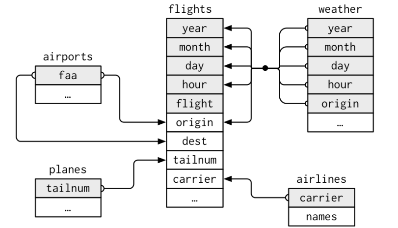
Relational data

flights connects to planes via tailnum variable.
flights connects to airlines via carrier variable.
flights connects to airports via the origin and dest variables.
flights connects to weather via origin, year, month, day and hour variables.

# Check variables in each tibble
library(tidyverse)
library(nycflights13)
flights
airlines
airports
planes
weather

Relational data

To connect each pair of tables we use unique identifiers called keys.

primary key - uniquely identifies an observation in its own table.
foreign key - uniquely identifies an observation in another table.
A variable can be both a primary key and a foreign key.
A primary key and the corresponding foreign key in another table form a relation
Relations are typically one-to-many.

Relational data

Use dm package to get some details about the data set.

library(dm)
dm <- dm_nycflights13(cycle = TRUE)
dm %>%
  dm_draw()

To get details all primary keys use the following:

#To get all primary keys
dm %>%
  dm_get_all_pks()

# A tibble: 4 x 2
  table    pk_col           
  <chr>    <keys>           
1 airlines carrier          
2 airports faa              
3 planes   tailnum          
4 weather  origin, time_hour

Use the following codes to check the suitability of each variable of a data set to serve as a primary key.

dm %>%
  dm_enum_pk_candidates(airports)

# A tibble: 8 x 3
  columns candidate why                                                         
  <keys>  <lgl>     <chr>                                                       
1 faa     TRUE      ""                                                          
2 name    TRUE      ""                                                          
3 lat     TRUE      ""                                                          
4 lon     TRUE      ""                                                          
5 alt     FALSE     "has duplicate values: 30 (4), 13 (3), 9 (2), 19 (2), 26 (2~
6 tz      FALSE     "has duplicate values: -5 (48), -6 (21), -8 (12), -7 (4)"   
7 dst     FALSE     "has duplicate values: A (84), N (2)"                       
8 tzone   FALSE     "has duplicate values: America/New_York (48), America/Chica~

We can identify foreign keys by using the function dm_enum_fk_candidates().

dm %>%
  dm_enum_fk_candidates(flights, airlines)

# A tibble: 19 x 3
   columns        candidate why                                                 
   <keys>         <lgl>     <chr>                                               
 1 carrier        TRUE      ""                                                  
 2 year           FALSE     "Can't combine `value1` <integer> and `value1` <cha~
 3 month          FALSE     "Can't combine `value1` <integer> and `value1` <cha~
 4 day            FALSE     "Can't combine `value1` <integer> and `value1` <cha~
 5 dep_time       FALSE     "Can't combine `value1` <integer> and `value1` <cha~
 6 sched_dep_time FALSE     "Can't combine `value1` <integer> and `value1` <cha~
 7 dep_delay      FALSE     "Can't combine `value1` <double> and `value1` <char~
 8 arr_time       FALSE     "Can't combine `value1` <integer> and `value1` <cha~
 9 sched_arr_time FALSE     "Can't combine `value1` <integer> and `value1` <cha~
10 arr_delay      FALSE     "Can't combine `value1` <double> and `value1` <char~
11 flight         FALSE     "Can't combine `value1` <integer> and `value1` <cha~
12 tailnum        FALSE     "values of `flights$tailnum` not in `airlines$carri~
13 origin         FALSE     "values of `flights$origin` not in `airlines$carrie~
14 dest           FALSE     "values of `flights$dest` not in `airlines$carrier`~
15 air_time       FALSE     "Can't combine `value1` <double> and `value1` <char~
16 distance       FALSE     "Can't combine `value1` <double> and `value1` <char~
17 hour           FALSE     "Can't combine `value1` <double> and `value1` <char~
18 minute         FALSE     "Can't combine `value1` <double> and `value1` <char~
19 time_hour      FALSE     "Can't combine `value1` <datetime<America/New_York>~

We can extract a summary of all foreign key relations present in a dm object using dm_get_all_fks():

dm %>% 
  dm_get_all_fks()

# A tibble: 5 x 5
  child_table child_fk_cols     parent_table parent_key_cols   on_delete
  <chr>       <keys>            <chr>        <keys>            <chr>    
1 flights     carrier           airlines     carrier           no_action
2 flights     origin            airports     faa               no_action
3 flights     dest              airports     faa               no_action
4 flights     tailnum           planes       tailnum           no_action
5 flights     origin, time_hour weather      origin, time_hour no_action

Relational data

Now, we select only 6 variables from flights data set to work with easily, and name it as flights2.

flights2 <- flights %>% 
  select(year:day, hour, tailnum, carrier)
flights2

Then, to add the full airline name, we combine the airlines and flights2 data tables using left_join() function.

flights2 %>%
   left_join(airlines, by = "carrier")

Refer more details: https://r4ds.had.co.nz/relational-data.html

Relational data

Suppose we have two data tables x and y.

inner_join(x,y) - keeps observations common to xand y.
left_join(x,y) - keeps all observations in x.
right_join(x,y) - keeps all observations in y.
full_join(x,y) - keeps all observations in x and y.
semi_join(x, y) - keeps all observations in x that have a match in y.
anti_join(x, y) - drops all observations in x that have a match in y.

Class work

Create two data sets student_residence and student_transport as below:

# Creating student_residence data set
set.seed(123)
student_residence <- data.frame(student = seq(1, 6),
distance = runif(6, 3, 10))
# Creating student_transport data set 
student_transport <- data.frame(student = seq(1, 7, by = 2),transport = c("Bus", "Carpool", "Walk", "Bus"))

Using dplyr package, apply inner_join(), left_join(), right_join() and full_join() to the above data sets, and interpret the results.

Must learn

Modeling Relational Data in R with ReDaMoR: https://cran.r-project.org/web/packages/ReDaMoR/vignettes/ReDaMoR.html#1_Introduction

The datamodelr R package provides tools to document relational data.

Importing data from Relational Databases: https://www.projectpro.io/data-science-in-r-programming-tutorial/r-tutorial-importing-data-from-relational-database

More Details

Data Carpentry, 2017-2018, dplyr package, https://datacarpentry.org/R-genomics/04-dplyr.html#data_manipulation_using_dplyr
dplyr : https://dplyr.tidyverse.org/
dplyr tutorial : https://www.listendata.com/2016/08/dplyr-tutorial.html
Data with dplyr : https://econ.suffolk.edu/dplyr/
dplyr flipbook: https://econ.suffolk.edu/slides/dplyr-summarize/#1
R for Data Science: https://r4ds.had.co.nz/relational-data.html
Relational data models: https://cran.rstudio.com/web/packages/dm/vignettes/howto-dm-theory.html

DSC 3091- Advanced Statistics Applications I

Data manipulation with dplyr

Data manipulation with dplyr

Data manipulation with dplyr

Data manipulation with dplyr

Data manipulation with dplyr

Data manipulation with dplyr

Data manipulation with dplyr

Data manipulation with dplyr

Data manipulation with dplyr

Class works

Class works

Relational data

Relational data

Relational data

Relational data

Relational data

Relational data

Relational data

Class work

Must learn

More Details

Data manipulation with `dplyr`

Data manipulation with `dplyr`

Data manipulation with `dplyr`

Data manipulation with `dplyr`

Data manipulation with `dplyr`

Data manipulation with `dplyr`

Data manipulation with `dplyr`

Data manipulation with `dplyr`

Data manipulation with `dplyr`