# A tibble: 150 x 5
   Sepal.Length Sepal.Width Petal.Length Petal.Width Species
          <dbl>       <dbl>        <dbl>       <dbl> <fct>
 1          5.1         3.5          1.4         0.2 setosa
 2          4.9         3            1.4         0.2 setosa
 3          4.7         3.2          1.3         0.2 setosa
 4          4.6         3.1          1.5         0.2 setosa
 5          5           3.6          1.4         0.2 setosa
 6          5.4         3.9          1.7         0.4 setosa
 7          4.6         3.4          1.4         0.3 setosa
 8          5           3.4          1.5         0.2 setosa
 9          4.4         2.9          1.4         0.2 setosa
10          4.9         3.1          1.5         0.1 setosa
# ... with 140 more rows
# i Use `print(n = ...)` to see more rowsDSC 3091- Advanced Statistics Applications I
Data Wrangling I
Department of Statistics and Computer Science
Data Wrangling
Data wrangling makes it easier to get your data into R in a useful form for visualisation and modelling. Here, we discuss the following three tools.
tibbles the variant of the data frame.
Data import in rectangular formats.
tidy data a consistent way of storing your data that makes transformation, visualisation, and modelling easier.
Tibbles
Tibbles are data frames, which makes easier for data wrangling. Tibbles can be created using the tibble package. Tibbles have an enhanced print() method which can be used with large datasets containing complex objects.
Tibbles
You can create a new tibble from individual vectors with tibble() function.
Tibbles vs. data.frame
Tibbles shows only the first 10 rows, and all the columns fit on screen, which makes it much easier to work with large data. In addition to its name, each column reports its data type.
tibble(
  a = lubridate::now(),
  b = lubridate::today(),
  c = 1:1e3,
  d = runif(1e3),
  e = sample(letters, 1e3, replace = TRUE)
)
# A tibble: 1,000 x 5
a b c d e
<dttm> <date> <int> <dbl> <chr>
1 2022-08-10 11:32:49 2022-08-10 1 0.302 i
2 2022-08-10 11:32:49 2022-08-10 2 0.619 g
3 2022-08-10 11:32:49 2022-08-10 3 0.475 u
4 2022-08-10 11:32:49 2022-08-10 4 0.387 b
5 2022-08-10 11:32:49 2022-08-10 5 0.468 s
6 2022-08-10 11:32:49 2022-08-10 6 0.723 q
7 2022-08-10 11:32:49 2022-08-10 7 0.416 m
8 2022-08-10 11:32:49 2022-08-10 8 0.607 z
9 2022-08-10 11:32:49 2022-08-10 9 0.893 z
10 2022-08-10 11:32:49 2022-08-10 10 0.994 a
# ... with 990 more rows
# i Use `print(n = ...)` to see more rowsTibbles vs. data.frame
Consider the below flights data set which shows on-time data for all flights that departed NYC in 2013, in nycflights13 package. If you want to see only 5 observations, use the below code. The option width = Inf shows all variables.
# A tibble: 336,776 x 19
   year month   day dep_time sched_dep_time dep_delay arr_time sched_arr_time
  <int> <int> <int>    <int>          <int>     <dbl>    <int>          <int>
1  2013     1     1      517            515         2      830            819
2  2013     1     1      533            529         4      850            830
3  2013     1     1      542            540         2      923            850
4  2013     1     1      544            545        -1     1004           1022
5  2013     1     1      554            600        -6      812            837
  arr_delay carrier flight tailnum origin dest  air_time distance  hour minute
      <dbl> <chr>    <int> <chr>   <chr>  <chr>    <dbl>    <dbl> <dbl>  <dbl>
1        11 UA        1545 N14228  EWR    IAH        227     1400     5     15
2        20 UA        1714 N24211  LGA    IAH        227     1416     5     29
3        33 AA        1141 N619AA  JFK    MIA        160     1089     5     40
4       -18 B6         725 N804JB  JFK    BQN        183     1576     5     45
5       -25 DL         461 N668DN  LGA    ATL        116      762     6      0
  time_hour
  <dttm>
1 2013-01-01 05:00:00
2 2013-01-01 05:00:00
3 2013-01-01 05:00:00
4 2013-01-01 05:00:00
5 2013-01-01 06:00:00
# ... with 336,771 more rows
# i Use `print(n = ...)` to see more rows
Tibbles vs. data.frame
To see the data in the default output of a tibble, use the below codes:
# A tibble: 336,776 x 19
    year month   day dep_time sched_dep_time dep_delay arr_time sched_arr_time
   <int> <int> <int>    <int>          <int>     <dbl>    <int>          <int>
 1  2013     1     1      517            515         2      830            819
 2  2013     1     1      533            529         4      850            830
 3  2013     1     1      542            540         2      923            850
 4  2013     1     1      544            545        -1     1004           1022
 5  2013     1     1      554            600        -6      812            837
 6  2013     1     1      554            558        -4      740            728
 7  2013     1     1      555            600        -5      913            854
 8  2013     1     1      557            600        -3      709            723
 9  2013     1     1      557            600        -3      838            846
10  2013     1     1      558            600        -2      753            745
   arr_delay carrier flight tailnum origin dest  air_time distance  hour minute
       <dbl> <chr>    <int> <chr>   <chr>  <chr>    <dbl>    <dbl> <dbl>  <dbl>
 1        11 UA        1545 N14228  EWR    IAH        227     1400     5     15
 2        20 UA        1714 N24211  LGA    IAH        227     1416     5     29
 3        33 AA        1141 N619AA  JFK    MIA        160     1089     5     40
 4       -18 B6         725 N804JB  JFK    BQN        183     1576     5     45
 5       -25 DL         461 N668DN  LGA    ATL        116      762     6      0
 6        12 UA        1696 N39463  EWR    ORD        150      719     5     58
 7        19 B6         507 N516JB  EWR    FLL        158     1065     6      0
 8       -14 EV        5708 N829AS  LGA    IAD         53      229     6      0
 9        -8 B6          79 N593JB  JFK    MCO        140      944     6      0
10         8 AA         301 N3ALAA  LGA    ORD        138      733     6      0
   time_hour
   <dttm>
 1 2013-01-01 05:00:00
 2 2013-01-01 05:00:00
 3 2013-01-01 05:00:00
 4 2013-01-01 05:00:00
 5 2013-01-01 06:00:00
 6 2013-01-01 05:00:00
 7 2013-01-01 06:00:00
 8 2013-01-01 06:00:00
 9 2013-01-01 06:00:00
10 2013-01-01 06:00:00
# ... with 336,766 more rows
# i Use `print(n = ...)` to see more rows
Data import
To read plain-text rectangular files into R, use the readr package, which is part of the core tidyverse.
read_csv()reads comma delimited files,read_csv2()reads semicolon separated files,read_tsv()reads tab delimited files, andread_delim()reads in files with any delimiter.read_fwf()reads fixed width files. You can specify fields either by their widths withfwf_widths()or their position withfwf_positions().read_table()reads a common variation of fixed width files where columns are separated by white space.
Data import
read_log()reads Apache style log files. (But also check out webreadr which is built on top ofread_log()and provides many more helpful tools.)
Suppose you have a csv file named heights in a folder called data. Then, to read it use
heights<-read_csv("data/heights.csv")
If some meta data included in the first two lines of the data set, and you want to skip those two lines, use
heights<-read_csv("data/heights.csv", skip=2)
Data import
Example
library(readr)
read_csv("The first line of metadata
  The second line of metadata
  x,y,z
  1,2,3", skip = 2)
# A tibble: 1 x 3
x y z
<dbl> <dbl> <dbl>
1 1 2 3If there is a comment in the data set,use the below codes:
Data import
If the variable names are not included in the data set, you can specify them and read the data as
heights<-read_csv("data/heights.csv", col_names = c("x", "y", "z"))
If the missing values are indicated as “.” in the data set, you can change them to NA as below:
heights<-read_csv("data/heights.csv", NA= ".")
Data import
If you data contains other characters such as $100, 20% or etc, then to convert them to data use parse_number() function.
Examples
Data import
To write dates in a given format, you can use parse_date() function.
Data import
Date abbreviations
| Year |
|
| Month |
|
| Day | %d - (2 digits) |
Tidy Data
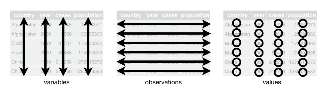
In tidy data
each variable forms a column
each observation forms a row
each cell is a single measurement
When working with tidy data, we can use the same tools in similar ways for different data sets.
dplyr, ggplot2, and all the other packages in the tidyverse are designed to work with tidy data.
Tidy Data

Tidy Data
What are the advantages of your data to be tidy?
The general advantage is that you can select one consistent way to store your data. If you have a consistent data structure, it’s easier to learn the tools that work with it since they have an underlying uniformity.
When variables are in columns, you can use the vectorised nature of R. Most of the built-in R functions work with vectors of values.
Tidy Data
Run the following codes and identify which data set/s is/are tidy.
These are all representations of the same underlying data, but only table1 is tidy.
Tidy Data
Examples
Run the following codes.
Tidy Data
If we have untidy data, how do we make them tidy?
To do this, you can use the functions pivot_longer() and pivot_wider() in tidyr.
# A tibble: 3 x 3
  country     `1999` `2000`
* <chr>        <int>  <int>
1 Afghanistan    745   2666
2 Brazil       37737  80488
3 China       212258 213766
Here, the column names 1999 and 2000 represent values of the year variable, and the values of these columns represent values of the cases variable. Note that each row represents two observations, but not one.
Tidy Data
Since one variable spreads across multiple columns in table4a , we use pivot_longer() function to make it tidy as below:
Tidy Data
In table2 data set, one observation is scattered across multiple rows. Therefore, we have to use pivot_wider() function to make it tidy.
# A tibble: 12 x 4
   country      year type            count
   <chr>       <int> <chr>           <int>
 1 Afghanistan  1999 cases             745
 2 Afghanistan  1999 population   19987071
 3 Afghanistan  2000 cases            2666
 4 Afghanistan  2000 population   20595360
 5 Brazil       1999 cases           37737
 6 Brazil       1999 population  172006362
 7 Brazil       2000 cases           80488
 8 Brazil       2000 population  174504898
 9 China        1999 cases          212258
10 China        1999 population 1272915272
11 China        2000 cases          213766
12 China 2000 population 1280428583# A tibble: 6 x 4
country year cases population
<chr> <int> <int> <int>
1 Afghanistan 1999 745 19987071
2 Afghanistan 2000 2666 20595360
3 Brazil 1999 37737 172006362
4 Brazil 2000 80488 174504898
5 China 1999 212258 1272915272
6 China 2000 213766 1280428583Tidy Data
In the following data set, we can separate the rate variables to two variables.
We separate the rate variables to cases and population variables.
# A tibble: 6 x 4
  country      year  cases population
  <chr>       <int>  <int>      <int>
1 Afghanistan  1999    745   19987071
2 Afghanistan  2000   2666   20595360
3 Brazil       1999  37737  172006362
4 Brazil       2000  80488  174504898
5 China        1999 212258 1272915272
6 China        2000 213766 1280428583
Tidy Data
We can also use sep option with separate function to separate integers.
# A tibble: 6 x 4
  country     century year  rate
  <chr>       <chr>   <chr> <chr>
1 Afghanistan 19      99    745/19987071
2 Afghanistan 20      00    2666/20595360
3 Brazil      19      99    37737/172006362
4 Brazil      20      00    80488/174504898
5 China       19      99    212258/1272915272
6 China       20      00    213766/1280428583
Tidy Data
Using unite() function we can combine multiple columns into a single column.
Now, we use unite() function to rejoin the century and year columns that we created in the previous example.
library(tidyverse)
table5<-table3 %>%
  separate(year, into = c("century", "year"), sep = 2)
table5 %>%
  unite(new, century, year, sep = "")# Run without sep="" option, and see the difference
# A tibble: 6 x 3
country new rate
<chr> <chr> <chr>
1 Afghanistan 1999 745/19987071
2 Afghanistan 2000 2666/20595360
3 Brazil 1999 37737/172006362
4 Brazil 2000 80488/174504898
5 China 1999 212258/1272915272
6 China 2000 213766/1280428583Tidy Data (Missing values)
A value can be missing in two ways, Explicitly (i.e. flagged with NA), Implicitly (i.e. simply not present in the data).
In this data set, the return for the fourth quarter of 2015 is explicitly missing, and the return for the first quarter of 2016 is implicitly missing
# A tibble: 7 x 3
   year   qtr return
  <dbl> <dbl>  <dbl>
1  2015     1   1.88
2  2015     2   0.59
3  2015     3   0.35
4  2015     4  NA
5  2016     2   0.92
6  2016     3   0.17
7  2016     4   2.66
Tidy Data
To make missing values explicit in tidy data, we can use complete() function.
Class work
Make
table4bdata set tidy, and combine it withtable4adata set.Refer the case study (12.6) shown in https://r4ds.had.co.nz/tidy-data.html, and understand the tools that we need to use for a real data set. Apply those tools to the COVID-19 confirmed data from John Hopkins University. You can access the data using the following codes:
library(readr)
confirmed<-read_csv("https://raw.githubusercontent.com/CSSEGISandData/COVID-19/master/csse_covid_19_data/csse_covid_19_time_series/time_series_covid19_confirmed_global.csv")
head(confirmed)
Some Useful Links …
Wickham, H (2014). Tidy Data. Journal of Statistical Software 58 (10). jstatsoft.org/v59/i10/
Grolemund, G & Wickham, H (2016). R for Data Science, https://r4ds.had.co.nz
Introduction to Tidy Data in R: https://stat2labs.sites.grinnell.edu/Handouts/rtutorials/IntroTidyData.html
tidyr: https://tidyr.tidyverse.org/
A ModernDive into R and the Tidyverse: https://moderndive.com/index.html