  N Th Age Sex R1 R2 R3 R4
1 1  1  28   1  4  4  4  4
2 2  1  32   1  4  4  4  4
3 3  1  41   1  3  3  3  3
4 4  2  21   1  4  3  3  2
5 5  2  34   1  4  3  3  2
6 6 1 24 1 3 3 3 2DSC 3091- Advanced Statistics Applications I
Categorical Data Analysis
Dr Jagath Senarathne
Department of Statistics and Computer Science
Categorical data
A categorical variable has a measurement scale consisting of a set of categories.
Examples:
choice of accommodation: house, condominium, and apartment.
political ideology: liberal, moderate, or conservative.
Gender: male and female
Categorical variables can be classified as Binary, Nominal or Ordinal.
Probability distributions for categorical data:
Binomial distribution
Multinomial distribution
Summarizing Categorical data
Example 1
Let’s consider the knee dataset in catdata R-packge.
Description:
In a clinical study n=127 patients with sport related injuries have been treated with two different therapies (chosen by random design). After 3,7 and 10 days of treatment the pain occuring during knee movement was observed.
- Check the structure of the data
'data.frame':   127 obs. of  8 variables:
 $ N  : int  1 2 3 4 5 6 7 8 9 10 ...
 $ Th : int  1 1 1 2 2 1 2 2 2 1 ...
 $ Age: int  28 32 41 21 34 24 28 40 24 39 ...
 $ Sex: num  1 1 1 1 1 1 1 1 0 0 ...
 $ R1 : int  4 4 3 4 4 3 4 3 4 4 ...
 $ R2 : int  4 4 3 3 3 3 3 2 4 4 ...
 $ R3 : int  4 4 3 3 3 3 3 2 4 4 ...
$ R4 : int 4 4 3 2 2 2 2 2 3 3 ...- Convert into factor variables
'data.frame':   127 obs. of  8 variables:
 $ N  : int  1 2 3 4 5 6 7 8 9 10 ...
 $ Th : Factor w/ 2 levels "1","2": 1 1 1 2 2 1 2 2 2 1 ...
 $ Age: int  28 32 41 21 34 24 28 40 24 39 ...
 $ Sex: Factor w/ 2 levels "0","1": 2 2 2 2 2 2 2 2 1 1 ...
 $ R1 : int  4 4 3 4 4 3 4 3 4 4 ...
 $ R2 : int  4 4 3 3 3 3 3 2 4 4 ...
 $ R3 : int  4 4 3 3 3 3 3 2 4 4 ...
$ R4 : int 4 4 3 2 2 2 2 2 3 3 ...- Changing factor levels
  N        Th Age    Sex R1 R2 R3 R4
1 1   Placebo  28 Female  4  4  4  4
2 2   Placebo  32 Female  4  4  4  4
3 3   Placebo  41 Female  3  3  3  3
4 4 Treatment  21 Female  4  3  3  2
5 5 Treatment  34 Female  4  3  3  2
6 6 Placebo 24 Female 3 3 3 2- Creating tabulated summaries
- Using
CrossTablefunction ingmodelspackage
   Cell Contents
|-------------------------|
|                       N |
| Chi-square contribution |
|           N / Row Total |
|           N / Col Total |
|         N / Table Total |
|-------------------------|


Total Observations in Table:  127


             |
             |      Male |    Female | Row Total |
-------------|-----------|-----------|-----------|
     Placebo |        17 |        46 |        63 |
             |     0.182 |     0.078 |           |
             |     0.270 |     0.730 |     0.496 |
             |     0.447 |     0.517 |           |
             |     0.134 |     0.362 |           |
-------------|-----------|-----------|-----------|
   Treatment |        21 |        43 |        64 |
             |     0.179 |     0.076 |           |
             |     0.328 |     0.672 |     0.504 |
             |     0.553 |     0.483 |           |
             |     0.165 |     0.339 |           |
-------------|-----------|-----------|-----------|
Column Total |        38 |        89 |       127 |
             |     0.299 |     0.701 |           |
-------------|-----------|-----------|-----------|
Categorical data visualization
Chi-square goodness of fit test
A statistical hypothesis test used to determine whether a variable is likely to come from a specified distribution or not.
In Knee injuries dataset, let’s check whether the patients were randomly allocated to the treatment and placebo groups.
- Null hypothesis: \(P_{trt}=P_{plc}=0.5\)
Treatment   Placebo
      0.5       0.5
     Chi-square test against specified probabilities

Data variable:   knee$Th

Hypotheses:
   null:        true probabilities are as specified
   alternative: true probabilities differ from those specified

Descriptives:
          observed freq. expected freq. specified prob.
Placebo               63           63.5             0.5
Treatment             64           63.5             0.5

Test results:
   X-squared statistic:  0.008
   degrees of freedom:  1
   p-value:  0.929
Chi-square test of Independence
A hypothesis test used to determine whether two categorical or nominal variables are likely to be related or not.
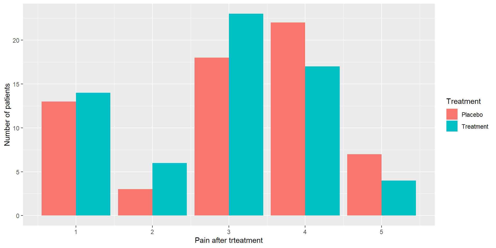
In Knee injuries dataset, let’s check whether the variables Th and R2 are independent or not.
     Chi-square test of categorical association

Variables:   Th, R2

Hypotheses:
   null:        variables are independent of one another
   alternative: some contingency exists between variables

Observed contingency table:
           R2
Th           1  2  3  4  5
  Placebo   13  3 18 22  7
  Treatment 14  6 23 17  4

Expected contingency table under the null hypothesis:
           R2
Th             1    2    3    4    5
  Placebo   13.4 4.46 20.3 19.3 5.46
  Treatment 13.6 4.54 20.7 19.7 5.54

Test results:
   X-squared statistic:  3.098
   degrees of freedom:  4
   p-value:  0.542

Other information:
   estimated effect size (Cramer's v):  0.156
   warning: expected frequencies too small, results may be inaccurate
Another way to do chi-square tests in R
- goodness of fit
    Chi-squared test for given probabilities

data:  table(knee$Th)
X-squared = 0.007874, df = 1, p-value = 0.9293- Independence
Assumptions of chi-square test
Expected frequencies are sufficiently large.
If this assumption is violated
If your expected cell counts are too small, check out the Fisher exact test.
observations are independent.
If observations are not independent
It may be possible to use the McNemar test or the Cochran test.
Fisher exact test
The Fisher exact test works somewhat differently to the chi-square test (or in fact any of the other hypothesis tests)
As can be seen it does not calculate a test statistic.
McNemar test
Suppose we want to check whether the two variables R2 and R3 are independent or not.
Here, both variables measure the pain of the same set of patients after the treatment.
Therefore, these observations can be correlated.
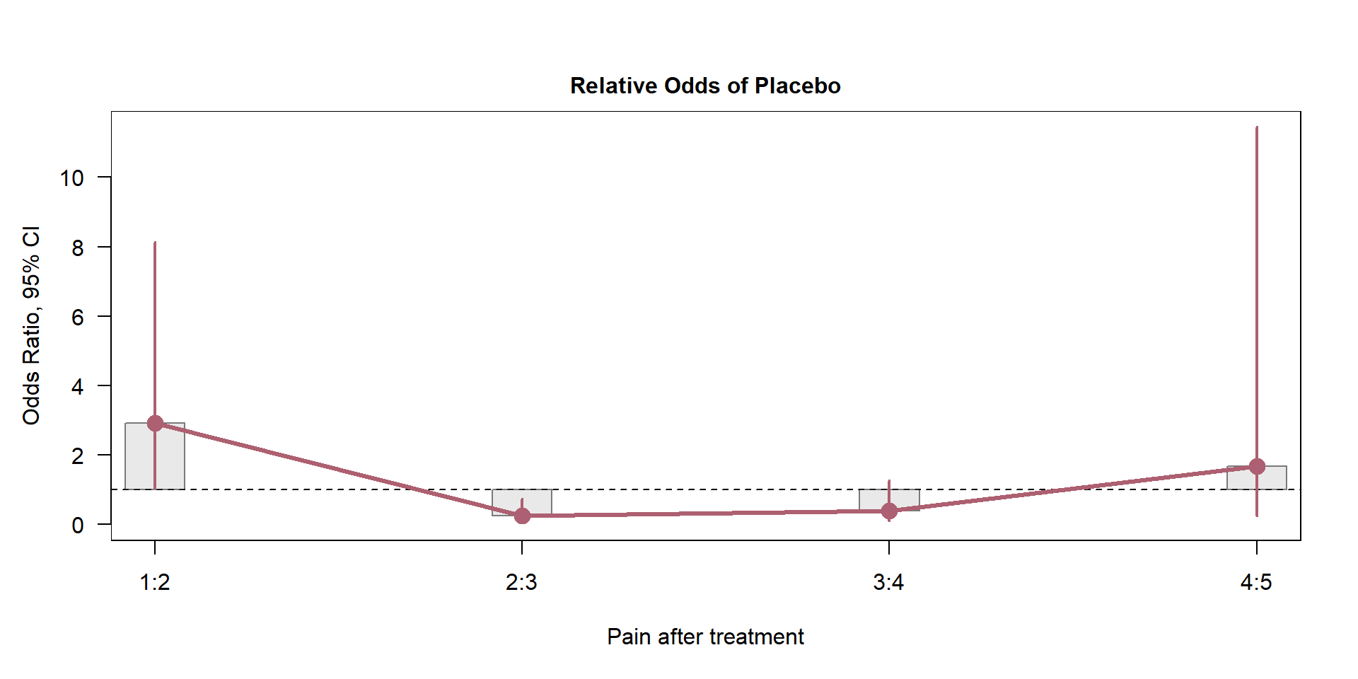
Odds Ratio and 95% CI
library(vcd) # install the package first
T5 <-table(knee$R4,knee$Th)
odds.2cb <- oddsratio(T5,log=F) # computes the odds ratio
summary(odds.2cb) # summary displays the odds ratio
z test of coefficients:

                      Estimate Std. Error z value Pr(>|z|)
1:2/Placebo:Treatment  2.90789    1.52468  1.9072  0.05649 .
2:3/Placebo:Treatment  0.24176    0.13799  1.7520  0.07978 .
3:4/Placebo:Treatment  0.38182    0.23506  1.6243  0.10430
4:5/Placebo:Treatment  1.66667    1.63865  1.0171  0.30911
---
Signif. codes: 0 '***' 0.001 '**' 0.01 '*' 0.05 '.' 0.1 ' ' 1- Plot the odds ratio and their respective confidence intervals.
Kendall rank correlation
Kendall rank correlation is used to test the similarities in the ordering of data.
A better alternative to Spearman correlation (non-parametric) when your sample size is small and has many tied ranks.
Example: Customer satisfaction (e.g. Very Satisfied, Somewhat Satisfied, Neutral.) and delivery time (< 30 Minutes, 30 minutes - 1 Hour, >2 Hours)
Some Useful Links …
https://www.r-bloggers.com/2022/01/handling-categorical-data-in-r-part-1/
https://towardsdatascience.com/kendall-rank-correlation-explained-dee01d99c535