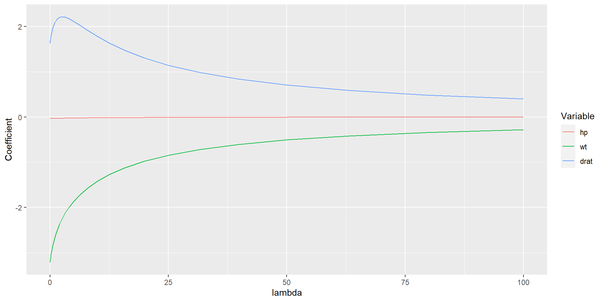
DSC 3091- Advanced Statistics Applications I

Penalized Regression and LARS algorithm

Dr Jagath Senarathne

Department of Statistics and Computer Science

Penalized Regression

  • Use the concept of penalizing or reducing the impact of certain variables in the model.

  • More suitable for large multivariate data sets containing a number of variables superior to the number of samples.

  • Also useful for selecting key variables from a large set of variables.

  • Penalized regression models improve prediction in new data by shrinking the size of coefficients and retaining those with coefficients greater than zero.

Penalized regression methods

  • Includes a penalty term to reduce (i.e. shrink) the coefficient values towards zero.

  • As such, the variables with minor contribution to the outcome have their coefficients close to zero.

  • Shrinkage methods:

    1. Ridge Regression

    2. Lasso Regression

    3. Elastic net Regression

Ridge Regression

  • We use ridge regression to tackle the multicollinearity problem.

  • Due to multicollinearity, the model estimates (least square) see a large variance.

  • Ridge regression is a method by which we add a degree of bias to the regression estimates.

  • Ridge regression performs L2 regularization which adds a penalty equivalent to the sum of the squared coefficients and tries to minimize them.

  • The ridge regression minimizes,

\(\sum(Y_i-\hat{Y}_i)^2+\lambda\sum{\beta_j^2}\)

Build a ridge regression model in r

  • To build the ridge regression in r, we use glmnet function from glmnet package in R.

Example

Let’s consider the mtcars dataset in R, and fit a ridge regression model to predict the mileage of the car.

library(glmnet)
x_var <- data.matrix(mtcars[, c("hp", "wt", "drat")])
y_var <- mtcars[, "mpg"]
lambda_seq <- 10^seq(2, -2, by = -.1)
fit <- glmnet(x_var, y_var, alpha = 0, lambda  = lambda_seq)
summary(fit)
          Length Class     Mode   
a0         41    -none-    numeric
beta      123    dgCMatrix S4     
df         41    -none-    numeric
dim         2    -none-    numeric
lambda     41    -none-    numeric
dev.ratio  41    -none-    numeric
nulldev     1    -none-    numeric
npasses     1    -none-    numeric
jerr        1    -none-    numeric
offset      1    -none-    logical
call        5    -none-    call   
nobs        1    -none-    numeric
# Get coefficients of all 100 models
ridge_coef <- coef(fit)

# Display coefficients for 7 models. 
round(ridge_coef[, c(1:3, 38:41)], 3)
4 x 7 sparse Matrix of class "dgCMatrix"
                s0     s1     s2    s37    s38    s39    s40
(Intercept) 20.092 20.100 20.112 29.271 29.293 29.313 29.329
hp          -0.004 -0.004 -0.005 -0.032 -0.032 -0.032 -0.032
wt          -0.281 -0.344 -0.418 -3.209 -3.212 -3.215 -3.218
drat         0.398  0.485  0.587  1.633  1.630  1.627  1.625
  • We can also produce a Trace plot to visualize how the coefficient estimates changed as a result of increasing \(\lambda\).
plot(fit, xvar ="lambda")

Choose an Optimal Value for \(\lambda\)

  • Identify the lambda value that produces the lowest mean squared error (MSE) by using k-fold cross-validation.

  • glmnet has the function cv.glmnet() that performs k-fold cross validation using k = 10 folds.

set.seed(123)
#perform k-fold cross-validation to find optimal lambda value
cv_model <- cv.glmnet(x_var, y_var, alpha = 0)

#find optimal lambda value that minimizes test MSE
best_lambda <- cv_model$lambda.min
best_lambda
[1] 1.08339

Plot of MSE by lambda value

plot(cv_model)

Final model

final_model <- glmnet(x_var, y_var, alpha = 0, lambda = best_lambda)
coef(final_model)
4 x 1 sparse Matrix of class "dgCMatrix"
                     s0
(Intercept) 25.49107983
hp          -0.03051333
wt          -2.63641838
drat         2.10130824

R-squared of the model

y_predicted <- predict(final_model, s = best_lambda, newx = x_var)

#find SST and SSE
sst <- sum((y_var - mean(y_var))^2)
sse <- sum((y_predicted - y_var)^2)

#find R-Squared
rsq <- 1 - sse/sst
rsq
[1] 0.8296018

Lasso regression

  • Lasso stands for Least Absolute Shrinkage and Selection Operator.

  • It shrinks the regression coefficients toward zero by penalizing the regression model with a penalty term called L1-norm.

\(\sum(Y_i-\hat{Y}_i)^2+\lambda\sum{|\beta_j|}\)

  • One advantage of lasso regression over ridge regression, is that it produces simpler and more interpretable models that incorporate only a reduced set of the predictors.

  • However, neither ridge regression nor the lasso will universally dominate the other.

  • Generally, lasso might perform better in a situation where some of the predictors have large coefficients, and the remaining predictors have very small coefficients.

  • Ridge regression will perform better when the outcome is a function of many predictors, all with coefficients of roughly equal size.

Computing lasso regression in R

# Find the best lambda using cross-validation
set.seed(123) 
cvl <- cv.glmnet(x_var, y_var, alpha = 1)
# Display the best lambda value
cvl$lambda.min
[1] 0.1034148
# Fit the final model on the training data
model_lasso <- glmnet(x_var, y_var, alpha = 1, lambda = cvl$lambda.min)
# Dsiplay regression coefficients
coef(model_lasso)
4 x 1 sparse Matrix of class "dgCMatrix"
                     s0
(Intercept) 29.63708800
hp          -0.03125498
wt          -3.21282109
drat         1.49439939

R-squared of the lasso regression model

y_predicted <- predict(model_lasso, s = cvl$lambda.min, newx = x_var)

#find SST and SSE
sst <- sum((y_var - mean(y_var))^2)
sse <- sum((y_predicted - y_var)^2)

#find R-Squared
rsq <- 1 - sse/sst
rsq
[1] 0.8364553

Elastic net regession

  • Elastic Net produces a regression model that is penalized with both the L1-norm and L2-norm.

  • The objective of this method is to effectively shrink coefficients (like in ridge regression) and to set some coefficients to zero (as in LASSO).

  • The elastic net regression can be easily computed using the caret workflow, which invokes the glmnet package.

  • The caret packages tests a range of possible alpha and lambda values, then selects the best values for lambda and alpha, resulting to a final model that is an elastic net model.

How to find alpha and lambda?

library(caret)
data.new <- data.frame(y_var,x_var)
set.seed(123)
model_ER <- train(
  y_var~.,data=data.new, method = "glmnet",
  trControl = trainControl("cv", number = 10),
  tuneLength = 10
)
# Best tuning parameter
model_ER$bestTune
  alpha   lambda
6   0.1 0.834975
  • Coefficient of the final model:
coef(model_ER$finalModel, model_ER$bestTune$lambda)
4 x 1 sparse Matrix of class "dgCMatrix"
                     s1
(Intercept) 26.44660083
hp          -0.03051303
wt          -2.74813181
drat         1.93555113

R-squared of the elastic net regression model

y_predicted <- predict(model_ER, newx = x_var)

#find SST and SSE
sst <- sum((y_var - mean(y_var))^2)
sse <- sum((y_predicted - y_var)^2)

#find R-Squared
rsq <- 1 - sse/sst
rsq
[1] 0.8312703

LARS algorithm

  • Least-angle regression (LARS) is an algorithm for fitting linear regression models to high-dimensional data.

  • It is a model selection method for linear regression.

  • At each step, LARS finds the attribute which is most highly correlated to the target value.

Algorithm

  1. Normalize all values to have zero mean and unit variance.

  2. Find a variable that is most highly correlated to the residual. Move the regression line in this direction until we reach another variable that has the same or higher correlation.

  3. When we have two variables that have the same correlation, move the regression line at an angle that is in between (i.e., least angle between the two variables).

  4. Continue this until all of our data is exhausted or until you think the model is big and ‘general’ enough.

Computing LARS model in R

  • Can use the lars function from lars package in R.

lars(x, y, type = c("lasso", "lar", "forward.stagewise", "stepwise"), trace = FALSE, normalize = TRUE, intercept = TRUE, Gram, eps = 1e-12, max.steps, use.Gram = TRUE)

Example

library(lars)
Lars_obj <- lars(x_var,y_var,type="lar")
Lars_obj

Call:
lars(x = x_var, y = y_var, type = "lar")
R-squared: 0.837 
Sequence of LAR moves:
     wt hp drat
Var   2  1    3
Step  1  2    3
plot(Lars_obj)

Advantages of using LARS:

  • Computationally as fast as forward selection but may sometimes be more accurate.

  • Numerically very efficient when the number of features is much larger than the number of data instances.

  • It can easily be modified to produce solutions for other estimators.

Disadvantages of using LARS:

  • LARS is highly sensitive to noise and can produce unpredictable results sometimes.

IN-CLASS ASSIGNMENT

Obtain a penalized regression model that best describes the variations in the response variable medv from the Boston dataset in MASS package.