DSC 3091- Advanced Statistics Applications I

Multiple Linear Regression

Dr Jagath Senarathne

Department of Statistics and Computer Science

Multiple Linear Regression

Studying the variation of Y(response variable) as a function of more than one X(explanatory) variables.
The general multiple linear regression model;

\[ Y= \beta_0+\beta_1x_1+\beta_2x_2...+\beta_px_p+ \epsilon\]

Where, \(\epsilon \sim N(0,\sigma^2)\) is the random noise component of the model and \(\beta_0,\beta_1,...,\beta_p\), are the unknown parameters.

Example 1

You might want to predict how well a stock will do based on some other information that you just happen to have.

Example 2

Imagine that you are a tourist guide. You need to provide the price range of food to your clients. The price of those food usually correlates with the Food Quality and Service Quality of the Restaurant.

Example 3

Imagine that you’re a traffic planner in your city and need to estimate the average commute time of drivers going from the east side of the city to the west. You know that it will depend on a number of factors like the distance driven, the number of stoplights on the route, and the number of other vehicles on the road.

How to fit a multiple linear regression model?

Steps you can follow:

Graphical Interpretation
Parameter Estimation
Tests on Parameters
Analysis of Variance
Interpretation and Prediction

Graphical Interpretation

Before fitting a multiple liner regression model, plot a scatterplot between every possible pair of variables.
It helps in visualizing the strength of relationships.
Can also be used for variable selection and identifying co-linearity.

Example

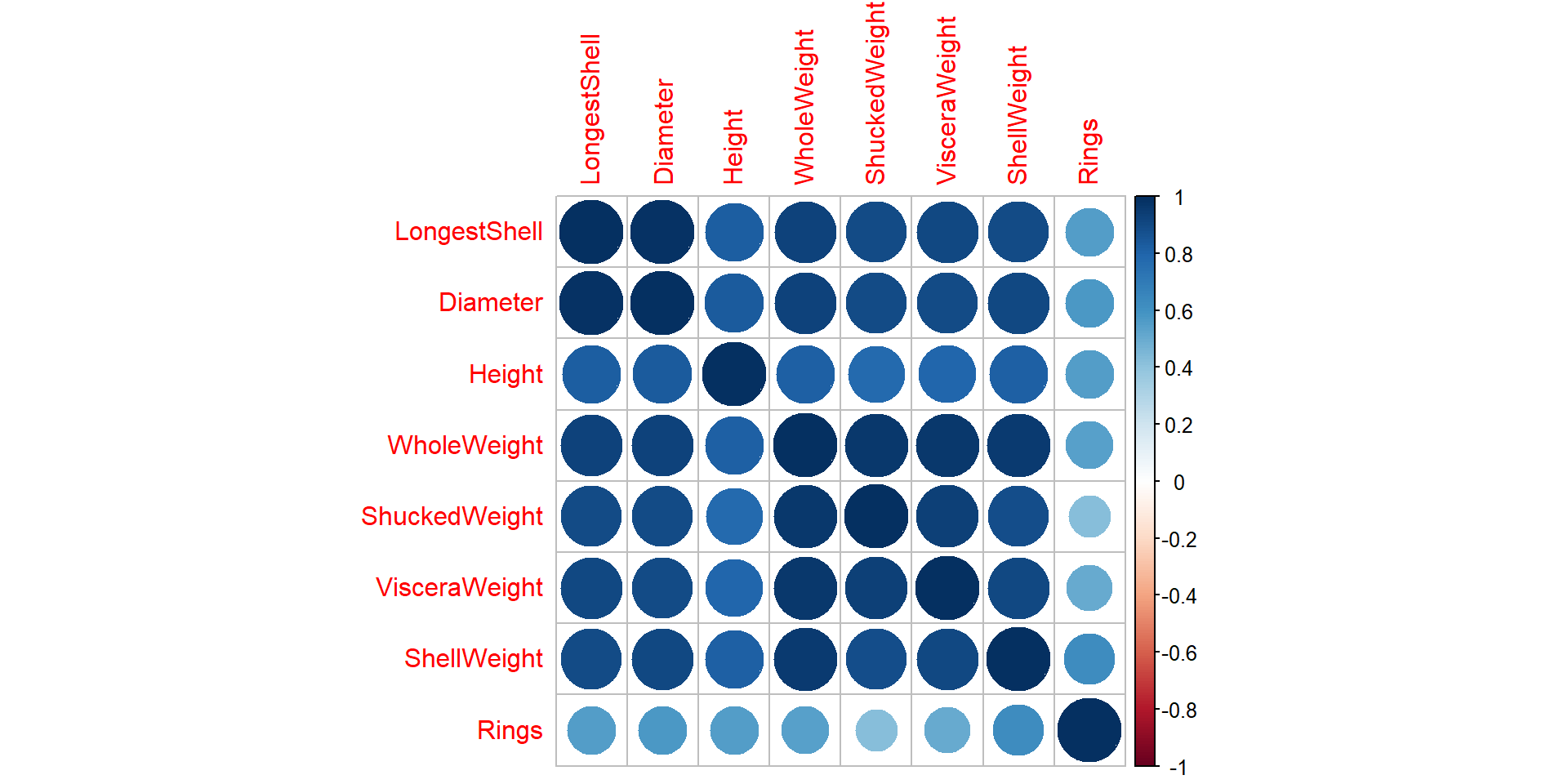
Let’s consider the built-in dataset, “abalone”, in the package called “AppliedPredictiveModeling”. Abalone data explains various physical measurements of sea snails. The main objective of this study is to predict the number of rings(which is an indicator of the age of the snail) using the other variables.

Example Cont…

install.packages("AppliedPredictiveModeling")
library(AppliedPredictiveModeling)
data(abalone)
attach(abalone)
head(abalone)
summary(abalone)
cor(abalone[,-1])

Draw a correlogram using corrplot() function

install.packages("corrplot")
library(corrplot)
corrplot(cor(abalone[,-1]), tl.col = "red")

Draw scatter plots using chart.Correlation():

#install.packages("PerformanceAnalytics")
library("PerformanceAnalytics")
chart.Correlation(abalone[,-1], histogram=TRUE, pch=19)

Parameter Estimation

Similar to the simple linear regression, we can use lm() function to estimate the unknown parameters \(\beta_0, \beta_1,.,\beta_p\).

model1 <-  lm(Rings~as.factor(Type) +LongestShell+ Diameter+ WholeWeight+ ShuckedWeight+ VisceraWeight+ ShellWeight)
model1


Call:
lm(formula = Rings ~ as.factor(Type) + LongestShell + Diameter + 
    WholeWeight + ShuckedWeight + VisceraWeight + ShellWeight)

Coefficients:
     (Intercept)  as.factor(Type)I  as.factor(Type)M      LongestShell  
         4.24786          -0.87919           0.04437          -0.05352  
        Diameter       WholeWeight     ShuckedWeight     VisceraWeight  
        12.73487           9.06362         -19.95631         -10.18938  
     ShellWeight  
         9.57238

summary(model1)


Call:
lm(formula = Rings ~ as.factor(Type) + LongestShell + Diameter + 
    WholeWeight + ShuckedWeight + VisceraWeight + ShellWeight)

Residuals:
    Min      1Q  Median      3Q     Max 
-8.1813 -1.3130 -0.3437  0.8690 13.7654 

Coefficients:
                  Estimate Std. Error t value Pr(>|t|)    
(Intercept)        4.24786    0.28883  14.707  < 2e-16 ***
as.factor(Type)I  -0.87919    0.10269  -8.562  < 2e-16 ***
as.factor(Type)M   0.04437    0.08380   0.529    0.597    
LongestShell      -0.05352    1.81860  -0.029    0.977    
Diameter          12.73487    2.22738   5.717 1.16e-08 ***
WholeWeight        9.06362    0.72947  12.425  < 2e-16 ***
ShuckedWeight    -19.95631    0.82169 -24.287  < 2e-16 ***
VisceraWeight    -10.18938    1.29997  -7.838 5.76e-15 ***
ShellWeight        9.57238    1.12490   8.510  < 2e-16 ***
---
Signif. codes:  0 '***' 0.001 '**' 0.01 '*' 0.05 '.' 0.1 ' ' 1

Residual standard error: 2.207 on 4168 degrees of freedom
Multiple R-squared:  0.5324,    Adjusted R-squared:  0.5315 
F-statistic: 593.3 on 8 and 4168 DF,  p-value: < 2.2e-16

Let’s create a dummy variable!

abalone$Type.I=ifelse(abalone$Type=="I",1,0)
abalone$Type.M=ifelse(abalone$Type=="M",1,0)
model2 <-  lm(Rings~Type.I + Type.M+ LongestShell+ Diameter+ WholeWeight+ ShuckedWeight+ VisceraWeight+ ShellWeight,data=abalone)
summary(model2)


Call:
lm(formula = Rings ~ Type.I + Type.M + LongestShell + Diameter + 
    WholeWeight + ShuckedWeight + VisceraWeight + ShellWeight, 
    data = abalone)

Residuals:
    Min      1Q  Median      3Q     Max 
-8.1813 -1.3130 -0.3437  0.8690 13.7654 

Coefficients:
               Estimate Std. Error t value Pr(>|t|)    
(Intercept)     4.24786    0.28883  14.707  < 2e-16 ***
Type.I         -0.87919    0.10269  -8.562  < 2e-16 ***
Type.M          0.04437    0.08380   0.529    0.597    
LongestShell   -0.05352    1.81860  -0.029    0.977    
Diameter       12.73487    2.22738   5.717 1.16e-08 ***
WholeWeight     9.06362    0.72947  12.425  < 2e-16 ***
ShuckedWeight -19.95631    0.82169 -24.287  < 2e-16 ***
VisceraWeight -10.18938    1.29997  -7.838 5.76e-15 ***
ShellWeight     9.57238    1.12490   8.510  < 2e-16 ***
---
Signif. codes:  0 '***' 0.001 '**' 0.01 '*' 0.05 '.' 0.1 ' ' 1

Residual standard error: 2.207 on 4168 degrees of freedom
Multiple R-squared:  0.5324,    Adjusted R-squared:  0.5315 
F-statistic: 593.3 on 8 and 4168 DF,  p-value: < 2.2e-16

Methods of building a multiple linear regression model

Backward Elimination
Forward Selection
Bidirectional Elimination (Stepwise regression)

Backward elimination

Set a significance level for which data will stay in the model.
Next, fit the full model with all possible predictors.
Consider the predictor with the highest P-value. If the P-value is greater than the significance level, you’ll move to step four, otherwise, you’re done!
Remove that predictor with the highest P-value.
Fit the model without that predictor variable.
Go back to step 3, do it all over, and keep doing that until you come to a point where even the highest P-value is < SL.

model2 <-  lm(Rings~Type.I + Type.M+ LongestShell+ Diameter+ WholeWeight+ ShuckedWeight+ VisceraWeight+ ShellWeight,data=abalone)
step.model <- step(model2, direction = "backward",trace=FALSE)
summary(step.model)


Call:
lm(formula = Rings ~ Type.I + Diameter + WholeWeight + ShuckedWeight + 
    VisceraWeight + ShellWeight, data = abalone)

Residuals:
    Min      1Q  Median      3Q     Max 
-8.1597 -1.3126 -0.3417  0.8697 13.7453 

Coefficients:
               Estimate Std. Error t value Pr(>|t|)    
(Intercept)     4.27930    0.26379  16.222  < 2e-16 ***
Type.I         -0.90566    0.08966 -10.101  < 2e-16 ***
Diameter       12.64787    0.94590  13.371  < 2e-16 ***
WholeWeight     9.06125    0.72926  12.425  < 2e-16 ***
ShuckedWeight -19.93199    0.81772 -24.375  < 2e-16 ***
VisceraWeight -10.22104    1.29262  -7.907 3.34e-15 ***
ShellWeight     9.57105    1.12421   8.514  < 2e-16 ***
---
Signif. codes:  0 '***' 0.001 '**' 0.01 '*' 0.05 '.' 0.1 ' ' 1

Residual standard error: 2.206 on 4170 degrees of freedom
Multiple R-squared:  0.5324,    Adjusted R-squared:  0.5317 
F-statistic: 791.3 on 6 and 4170 DF,  p-value: < 2.2e-16

Backward elimination using `SignifReg` package

library(SignifReg)
nullmodel = lm(Rings~1, data=abalone)
fullmodel = lm(Rings~Type.I + Type.M+ LongestShell+ Diameter+ WholeWeight+ ShuckedWeight+ VisceraWeight+ ShellWeight, data=abalone)
scope = list(lower=formula(nullmodel),upper=formula(fullmodel))

Sub.model=drop1SignifReg(fullmodel, scope, alpha = 0.05, criterion = "p-value",override="TRUE")
summary(Sub.model)


Call:
lm(formula = Rings ~ Type.I + Type.M + LongestShell + Diameter + 
    WholeWeight + VisceraWeight + ShellWeight, data = abalone)

Residuals:
    Min      1Q  Median      3Q     Max 
-8.7218 -1.4383 -0.4426  0.8413 16.3379 

Coefficients:
              Estimate Std. Error t value Pr(>|t|)    
(Intercept)    5.19685    0.30571  16.999  < 2e-16 ***
Type.I        -1.08469    0.10933  -9.921  < 2e-16 ***
Type.M        -0.07688    0.08937  -0.860   0.3897    
LongestShell  -3.36753    1.93732  -1.738   0.0822 .  
Diameter      13.40996    2.37930   5.636 1.85e-08 ***
WholeWeight   -5.61381    0.43643 -12.863  < 2e-16 ***
VisceraWeight -1.87624    1.33974  -1.400   0.1615    
ShellWeight   26.79546    0.93284  28.725  < 2e-16 ***
---
Signif. codes:  0 '***' 0.001 '**' 0.01 '*' 0.05 '.' 0.1 ' ' 1

Residual standard error: 2.357 on 4169 degrees of freedom
Multiple R-squared:  0.4663,    Adjusted R-squared:  0.4654 
F-statistic: 520.3 on 7 and 4169 DF,  p-value: < 2.2e-16

Forward selection

Choose the significance level (SL = 0.05).
Fit all possible simple regression models and select the one with the lowest P-value.
Keep this variable and fit all possible models with one extra predictor added to the one you already have.
Find the predictor with the lowest P-value. If P < Sl, go back to step 3. Otherwise, you’re done!

model2 <-  lm(Rings~Type.I + Type.M+ LongestShell+ Diameter+ WholeWeight+ ShuckedWeight+ VisceraWeight+ ShellWeight,data=abalone)
step.model2 <- step(model2, direction = "forward",trace=FALSE)
summary(step.model2)


Call:
lm(formula = Rings ~ Type.I + Type.M + LongestShell + Diameter + 
    WholeWeight + ShuckedWeight + VisceraWeight + ShellWeight, 
    data = abalone)

Residuals:
    Min      1Q  Median      3Q     Max 
-8.1813 -1.3130 -0.3437  0.8690 13.7654 

Coefficients:
               Estimate Std. Error t value Pr(>|t|)    
(Intercept)     4.24786    0.28883  14.707  < 2e-16 ***
Type.I         -0.87919    0.10269  -8.562  < 2e-16 ***
Type.M          0.04437    0.08380   0.529    0.597    
LongestShell   -0.05352    1.81860  -0.029    0.977    
Diameter       12.73487    2.22738   5.717 1.16e-08 ***
WholeWeight     9.06362    0.72947  12.425  < 2e-16 ***
ShuckedWeight -19.95631    0.82169 -24.287  < 2e-16 ***
VisceraWeight -10.18938    1.29997  -7.838 5.76e-15 ***
ShellWeight     9.57238    1.12490   8.510  < 2e-16 ***
---
Signif. codes:  0 '***' 0.001 '**' 0.01 '*' 0.05 '.' 0.1 ' ' 1

Residual standard error: 2.207 on 4168 degrees of freedom
Multiple R-squared:  0.5324,    Adjusted R-squared:  0.5315 
F-statistic: 593.3 on 8 and 4168 DF,  p-value: < 2.2e-16

Forward selection using `SignifReg` package

library(SignifReg)
nullmodel = lm(Rings~1, data=abalone)
fullmodel = lm(Rings~Type.I + Type.M+ LongestShell+ Diameter+ WholeWeight+ ShuckedWeight+ VisceraWeight+ ShellWeight, data=abalone)
scope = list(lower=formula(nullmodel),upper=formula(fullmodel))

sub.model2=add1SignifReg(nullmodel,scope, alpha = 0.05, criterion = "p-value",override="TRUE")
summary(sub.model2)


Call:
lm(formula = Rings ~ LongestShell, data = abalone)

Residuals:
    Min      1Q  Median      3Q     Max 
-5.9665 -1.6961 -0.7423  0.8733 16.6776 

Coefficients:
             Estimate Std. Error t value Pr(>|t|)    
(Intercept)    2.1019     0.1855   11.33   <2e-16 ***
LongestShell  14.9464     0.3452   43.30   <2e-16 ***
---
Signif. codes:  0 '***' 0.001 '**' 0.01 '*' 0.05 '.' 0.1 ' ' 1

Residual standard error: 2.679 on 4175 degrees of freedom
Multiple R-squared:  0.3099,    Adjusted R-squared:  0.3098 
F-statistic:  1875 on 1 and 4175 DF,  p-value: < 2.2e-16

Stepwise regression

Select a significance level to enter and a significance level to stay.
Perform the next step of forward selection where you add the new variable.
Now perform all of the steps of backward elimination.
Now head back to step two, then move forward to step 3, and so on until no new variables can enter and no new variables can exit.

model2 <-  lm(Rings~Type.I + Type.M+ LongestShell+ Diameter+ WholeWeight+ ShuckedWeight+ VisceraWeight+ ShellWeight,data=abalone)
step.model2 <- step(model2, direction = "forward", trace=FALSE)
summary(step.model2)


Call:
lm(formula = Rings ~ Type.I + Type.M + LongestShell + Diameter + 
    WholeWeight + ShuckedWeight + VisceraWeight + ShellWeight, 
    data = abalone)

Residuals:
    Min      1Q  Median      3Q     Max 
-8.1813 -1.3130 -0.3437  0.8690 13.7654 

Coefficients:
               Estimate Std. Error t value Pr(>|t|)    
(Intercept)     4.24786    0.28883  14.707  < 2e-16 ***
Type.I         -0.87919    0.10269  -8.562  < 2e-16 ***
Type.M          0.04437    0.08380   0.529    0.597    
LongestShell   -0.05352    1.81860  -0.029    0.977    
Diameter       12.73487    2.22738   5.717 1.16e-08 ***
WholeWeight     9.06362    0.72947  12.425  < 2e-16 ***
ShuckedWeight -19.95631    0.82169 -24.287  < 2e-16 ***
VisceraWeight -10.18938    1.29997  -7.838 5.76e-15 ***
ShellWeight     9.57238    1.12490   8.510  < 2e-16 ***
---
Signif. codes:  0 '***' 0.001 '**' 0.01 '*' 0.05 '.' 0.1 ' ' 1

Residual standard error: 2.207 on 4168 degrees of freedom
Multiple R-squared:  0.5324,    Adjusted R-squared:  0.5315 
F-statistic: 593.3 on 8 and 4168 DF,  p-value: < 2.2e-16

Model Diagnosis

The model fitting is just the first part of the regression analysis since this is all based on certain assumptions.
Regression diagnostics are used to evaluate the model assumptions and investigate whether or not there are observations with a large, undue influence on the analysis.

Model Assumptions

Before using a regression model for interpreting the data, we must check that the model assumptions are met.

Basic assumptions of regression models:

Linearity of the data: The relationship between the predictor (x) and the outcome (y) is assumed to be linear.
Normality of residuals: The residual errors are assumed to be normally distributed.
Homogeneity of residuals variance: The residuals are assumed to have a constant variance (homoscedasticity)
Independence of residuals error terms.

Checking Assumptions

par(mfrow = c(2, 2)) 
plot(step.model2)

Using `ggfortify` package

par(mfrow = c(2, 2)) 
library(ggfortify) 
autoplot(step.model2)

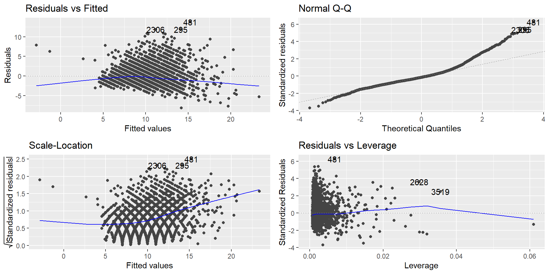
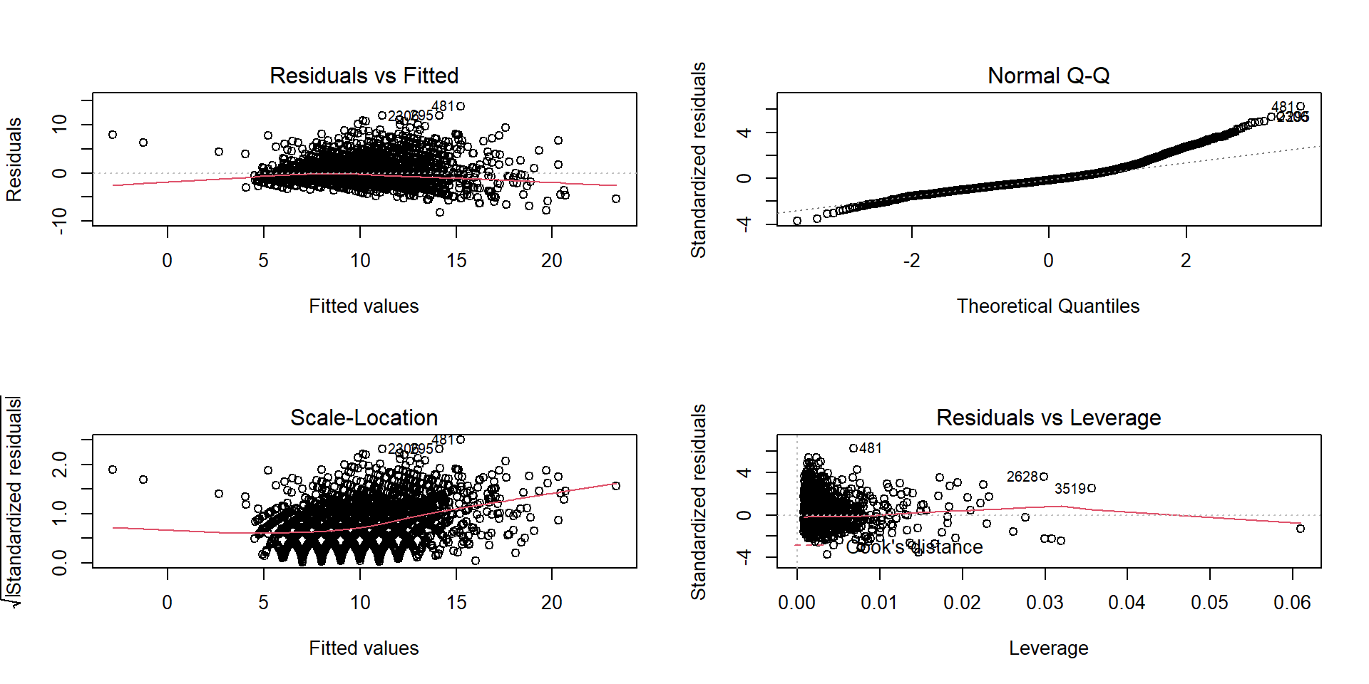
The diagnostic plots show residuals in four different ways:

Residuals vs Fitted: to check the linear relationship assumptions.
Normal Q-Q: to examine whether the residuals are normally distributed.
Scale-Location (or Spread-Location): to check the homogeneity of variance of the residuals (homoscedasticity).
Residuals vs Leverage: to identify extreme values that might influence the regression analysis.

Identifying Influential Outliers

An outlier is a point which is often distant from the others.
It is a point with a large value of its residual.
Different residual measures can be used to identify outliers.
- Standardised residuals
- Studentized residuals
- Cook’s distance

Standardised residuals

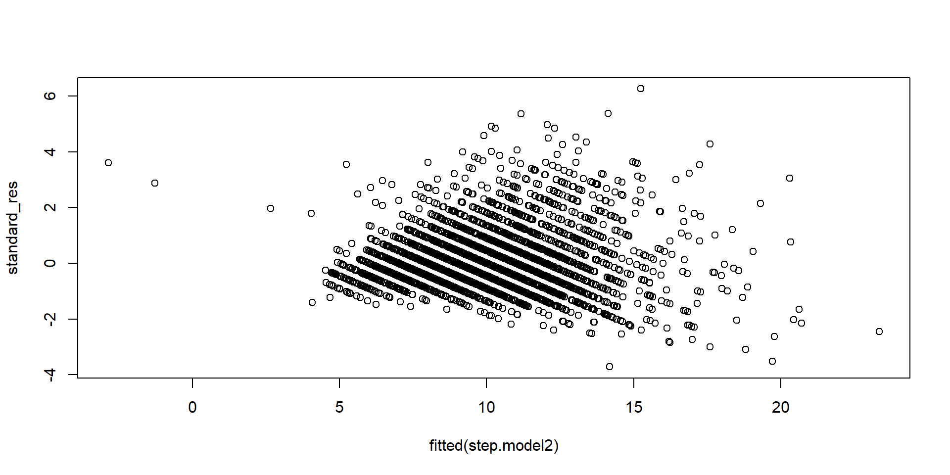
standard_res=rstandard(step.model2)
plot(fitted(step.model2), standard_res)

Standardized residuals are “mostly” between 2 and 2, but they are dependent.

Studentized residuals

student_res=rstudent(step.model2)
plot(fitted(step.model2), student_res)

For an outlier the absolute values of its Studentized residual is greater than the 0.975th quantile of the Student distribution with \(n-p-2\) degrees of freedom

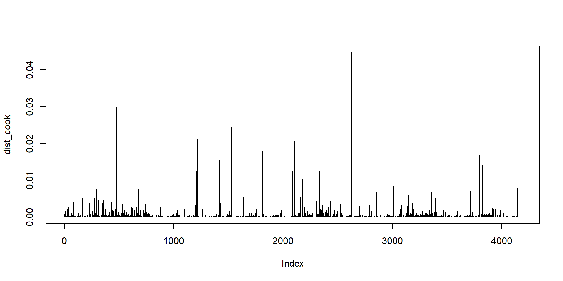
Cook’s Distance

It is calculated by removing the \(i\)th data point from the model and refitting the regression model.
It summarizes how much all the values in the regression model change when the \(i\)th observation is removed.
The formula for Cook’s distance is:
An R function to calculate Cook’s distance is cooks.distance().

dist_cook=cooks.distance(step.model2)
plot(dist_cook, type="h")

Checking for multicollinearity

It is a statistical terminology where more than one independent variable is correlated with each other.
Results in reducing the reliability of statistical inferences.
Hence, these variables must be removed when building a multiple regression model.
Variance inflation factor (VIF) is used for detecting the multicollinearity in a model.

Variance inflation factor

library(car)
vif_values <- vif(step.model2)          
barplot(vif_values, main = "VIF Values", horiz = TRUE, col = "steelblue") 
abline(v = 5, lwd = 3, lty = 2)

Testing the multicollinearity among the predictor variables

The mctest package in R provides the Farrar-Glauber test and other relevant tests for multicollinearity.

library(mctest)
omcdiag(mod=step.model2)


Call:
omcdiag(mod = step.model2)


Overall Multicollinearity Diagnostics

                       MC Results detection
Determinant |X'X|:         0.0000         1
Farrar Chi-Square:     62488.4404         1
Red Indicator:             0.7378         1
Sum of Lambda Inverse:   262.8746         1
Theil's Method:            2.8529         1
Condition Number:        104.1100         1

1 --> COLLINEARITY is detected by the test 
0 --> COLLINEARITY is not detected by the test

library(mctest)
imcdiag(mod=step.model2)


Call:
imcdiag(mod = step.model2)


All Individual Multicollinearity Diagnostics Result

                   VIF    TOL         Wi         Fi Leamer     CVIF Klein
Type.I          1.9723 0.5070   579.0942   675.7720 0.7120  -0.9408     0
Type.M          1.3975 0.7155   236.7649   276.2919 0.8459  -0.6666     0
LongestShell   40.9040 0.0244 23765.6736 27733.2698 0.1564 -19.5107     1
Diameter       41.9003 0.0239 24359.0324 28425.6879 0.1545 -19.9859     1
WholeWeight   109.7357 0.0091 64759.8525 75571.2838 0.0955 -52.3425     1
ShuckedWeight  28.5255 0.0351 16393.4264 19130.2517 0.1872 -13.6063     1
VisceraWeight  17.4123 0.0574  9774.6981 11406.5499 0.2396  -8.3054     1
ShellWeight    21.0270 0.0476 11927.5022 13918.7571 0.2181 -10.0296     1
                IND1   IND2
Type.I        0.0009 0.5994
Type.M        0.0012 0.3458
LongestShell  0.0000 1.1861
Diameter      0.0000 1.1868
WholeWeight   0.0000 1.2047
ShuckedWeight 0.0001 1.1732
VisceraWeight 0.0001 1.1460
ShellWeight   0.0001 1.1580

1 --> COLLINEARITY is detected by the test 
0 --> COLLINEARITY is not detected by the test

Type.M , LongestShell , coefficient(s) are non-significant may be due to multicollinearity

R-square of y on all x: 0.5324 

* use method argument to check which regressors may be the reason of collinearity
===================================

Model Selection

Model selection criteria refer to a set of exploratory tools for improving regression models.
Each model selection tool involves selecting a subset of possible predictor variables that still account well for the variation in the regression model’s response variable.
This suggests that we need a quality criteria that considers the size of the model, since our preference is for small models that still fit well.
Several criteria are available to measure the performance of model. (AIC, BIC , \(R^2\) (Coefficient of determination), adjacent \(R^2\))

The summary() function gives both \(R^2\) and adjacent \(R^2\) measures together.

summary(step.model2)


Call:
lm(formula = Rings ~ Type.I + Type.M + LongestShell + Diameter + 
    WholeWeight + ShuckedWeight + VisceraWeight + ShellWeight, 
    data = abalone)

Residuals:
    Min      1Q  Median      3Q     Max 
-8.1813 -1.3130 -0.3437  0.8690 13.7654 

Coefficients:
               Estimate Std. Error t value Pr(>|t|)    
(Intercept)     4.24786    0.28883  14.707  < 2e-16 ***
Type.I         -0.87919    0.10269  -8.562  < 2e-16 ***
Type.M          0.04437    0.08380   0.529    0.597    
LongestShell   -0.05352    1.81860  -0.029    0.977    
Diameter       12.73487    2.22738   5.717 1.16e-08 ***
WholeWeight     9.06362    0.72947  12.425  < 2e-16 ***
ShuckedWeight -19.95631    0.82169 -24.287  < 2e-16 ***
VisceraWeight -10.18938    1.29997  -7.838 5.76e-15 ***
ShellWeight     9.57238    1.12490   8.510  < 2e-16 ***
---
Signif. codes:  0 '***' 0.001 '**' 0.01 '*' 0.05 '.' 0.1 ' ' 1

Residual standard error: 2.207 on 4168 degrees of freedom
Multiple R-squared:  0.5324,    Adjusted R-squared:  0.5315 
F-statistic: 593.3 on 8 and 4168 DF,  p-value: < 2.2e-16

AIC(step.model2)

[1] 18477.14

library(lme4)
BIC(step.model2)

[1] 18540.52

Choose the model with lower AIC and BIC values.

In-Class Assignment

Obtain a multiple linear regression model that best describes the variations in the response variable Rings in the abalone dataset. Briefly discuss the steps you followed and the suitability of the model you selected.

DSC 3091- Advanced Statistics Applications I

Multiple Linear Regression

How to fit a multiple linear regression model?

Graphical Interpretation

Example Cont…

Draw a correlogram using corrplot() function

Draw scatter plots using chart.Correlation():

Parameter Estimation

Let’s create a dummy variable!

Methods of building a multiple linear regression model

Backward elimination

Backward elimination using SignifReg package

Forward selection

Forward selection using SignifReg package

Stepwise regression

Model Diagnosis

Model Assumptions

Checking Assumptions

Using ggfortify package

Identifying Influential Outliers

Standardised residuals

Studentized residuals

Cook’s Distance

Checking for multicollinearity

Variance inflation factor

Testing the multicollinearity among the predictor variables

Model Selection

In-Class Assignment

Some Useful Links …

Backward elimination using `SignifReg` package

Forward selection using `SignifReg` package

Using `ggfortify` package