DSC 3091- Advanced Statistics Applications I

Point Estimation and Confidence Intervals

Dr Jagath Senarathne

Department of Statistics and Computer Science

Point Estimation

Recall

• Parameter: Characteristics that are used to describe the population.

• Statistic: a function of the observable random variables in a sample which does not include any unknown quantities.

• Estimator: A statistic that is used to estimate an unknown parameter.

Point Estimation Cont…

Parameter	Estimator
Population mean \(\mu\)	Sample mean \(\bar{x}\)
Population variance \(\sigma^2\)	Sample variance \(s^2\)
Population proportion \(p\)	Sample proportion \(\hat{p}\)

Maximum Likelihood Estimators

• The point in the parameter space that maximizes the likelihood function.

• Likelihood function is given by; \[𝐿(𝑥,\theta)=\prod_{𝑖=1}^𝑛𝑓(𝑥_i,\theta)\]

• The idea of maximum likelihood estimation is to first assume our data come from a known family of distributions that contain parameters.

• Then the maximum likelihood estimates (MLEs) of the parameters will be the parameter values that are most likely to have generated our data.

Example 1

• Consider a simple coin-flipping example. Let’s say we flipped a coin 200 times and observed 103 heads and 97 tails. If the probability of “success” (i.e. getting a head) is \(p\),

  1. Define a function that will calculate the likelihood function for a given value of \(p\); then

  2. Search for the value of \(p\) that results in the highest likelihood.

Example 2

Suppose we have data points representing the weight (in kg) of students in a class.

 [1] 59.001 38.267 41.025 35.555 46.690 20.994 39.407 52.780 57.495 52.416
[11] 60.062 48.149 40.182 50.929 49.472 49.197 43.459 40.493 60.196 58.590
[21] 53.645 53.837 61.134 62.115 46.517 41.404 56.500 53.281 44.821 47.610
[31] 51.178 58.315 34.411 47.795 41.828 60.767 60.797 51.421 51.570 48.313
[41] 47.310 58.078 38.753 35.692 50.604 42.070 53.403 47.405 36.952 53.682

This dataset appears to follow a normal distribution. Find the MLEs for the mean and standard deviation for this distribution?

Normal distribution - Maximum Likelihood Estimation

• The MLE of \(\mu\) is defined as \(\hat{\mu}_{MLE}=argmax(x_1,...,x_n|\mu,\sigma^2)\); where \(\hat{\mu}_{MLE}\) is the value of \(\mu\) that maximizes the likelihood function.

• If we maximise the above likelihood function, we get \(\hat{\mu}_{MLE}=\bar{x}.\)

• Since the MLE of \(\mu\) is the sample mean, computing the MLE in R becomes straightforward.

Interval Estimation

• Point estimators are often use as sample measures for population parameters.

• It is also helpful to know how reliable this estimate is, that is, how much sampling uncertainty is associated with it.

• A useful way to express this uncertainty is to calculate an interval estimate or confidence interval for the population parameter

• In other words, the confidence interval is of the form “point estimate ± uncertainty”

Confidence Interval for Mean

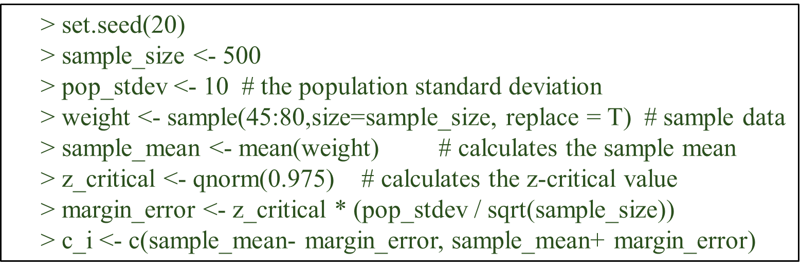
Case 1: When data is normal/ large sample and \(\sigma\) is known.

\[\bar{x}\pm z_{\alpha/2}\sigma/\sqrt{n}\]

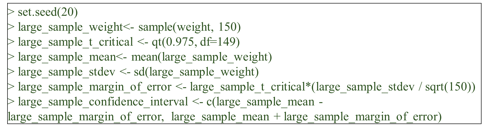
Case 2: When data is normal/ large samples and \(\sigma\) is unknown.

\[\bar{x}\pm t_{n-1,\alpha/2}\sigma/\sqrt{n}\]

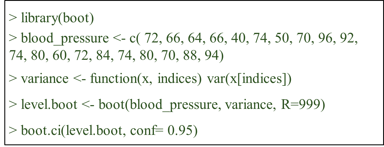
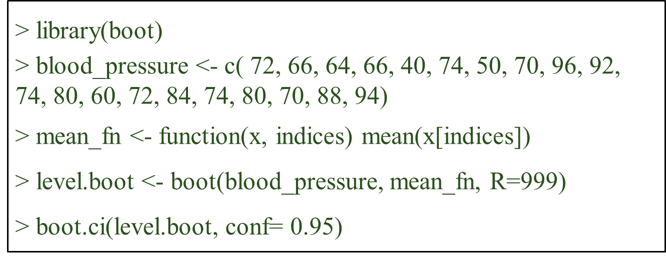
Case 3: When data is non-normal/ small samples

• For this, bootstrap approach is used as follows.

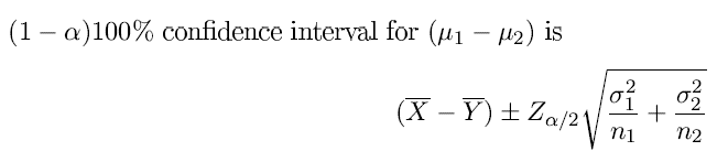
CONFIDENCE INTERVALS FOR Difference of Means

Case 1: Sampling from two independent normal distributions with known variances.

library("BSDA")
z.test(x,y = NULL,alternative = "two.sided",
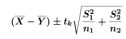
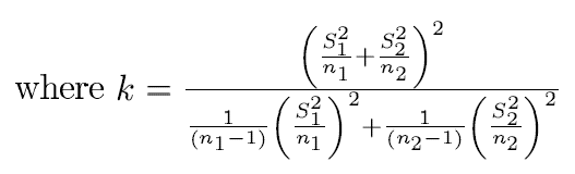
sigma.x = NULL, sigma.y = NULL, conf.level = 0.95)

Case 2: Sampling from two independent normal distributions with unknown variances (small samples).

• when population variances are equal

    t.test(x,y,alternative = "two.sided",
    var.equal=TRUE, conf.level = 0.95)

• when population variances are unequal

  t.test(x,y,alternative = "two.sided",
    var.equal=FALSE, conf.level = 0.95)

Confidence Interval Chart in R (Independent Means & CIs)

• Example

set.seed(123456)                 # Create example data
data <- data.frame(x = c("A","B","C"),
                  y = round(runif(3, 10, 20),2),
                  lower = round(runif(3, 0, 10),2),
                  upper = round(runif(3, 20, 30),2))

library(ggplot2)
ggplot(data, aes(x, y)) +        # ggplot2 plot with confidence intervals
  geom_point() +
  geom_errorbar(aes(ymin = lower, ymax = upper))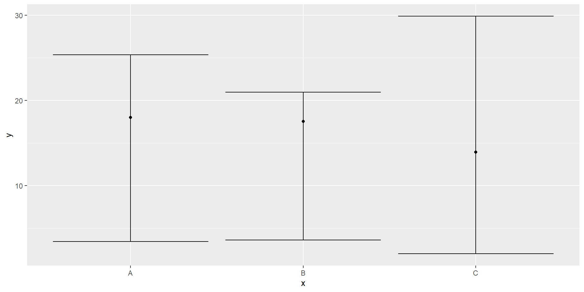

Confidence Intervals for Proportion

• Case 1: For large sample (Using Normal approximation)

\[ \hat{p}\pm Z_{\alpha/2}\sqrt{\frac{\hat{p}(1-\hat{p})}{n}}\]

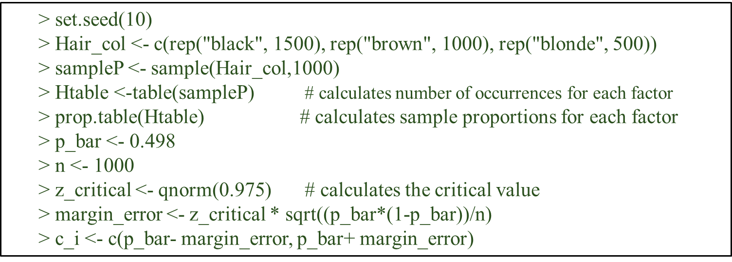
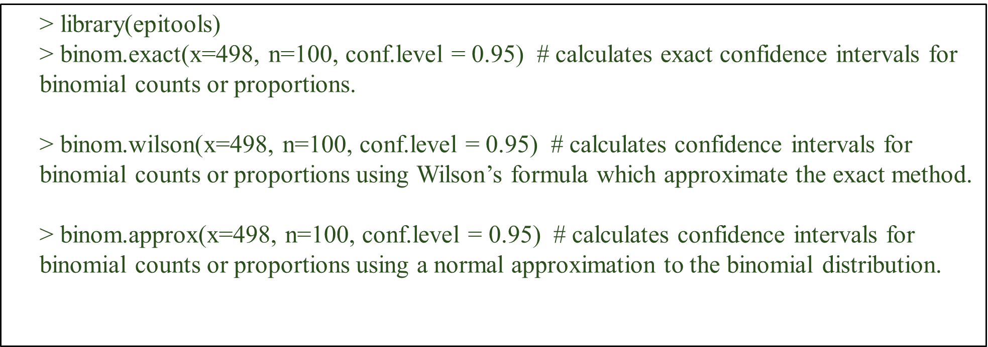
Case 1: For large sample (Using Binomial Distribution)

• we can use the following functions from R package epitools for this case.

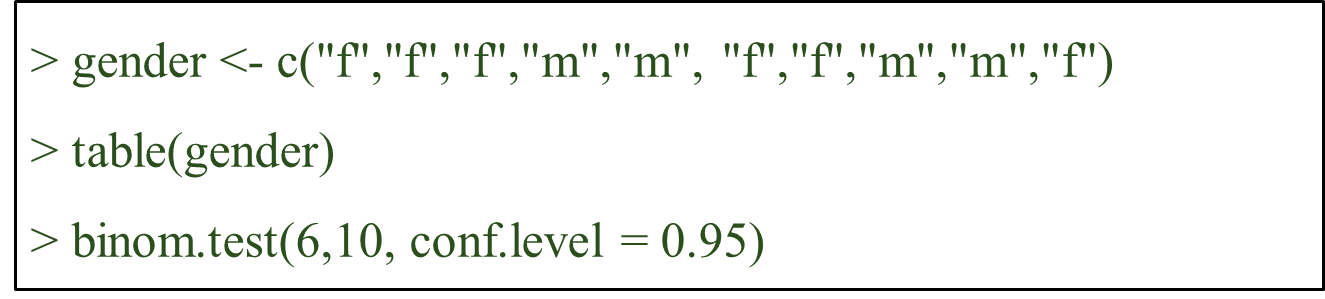
Case 2: For small sample (Using Binomial Distribution)

• When sample size is small, confidence interval for population can be calculated using binom.test() function.

Confidence Intervals for Variance

Case 1: Under normality assumption

• User defined function to obtain confidence interval for variance.

 var.interval = function(data, conf.level = 0.95) {
 df = length(data) - 1
 chilower = qchisq((1 - conf.level)/2, df)
 chiupper = qchisq((1 - conf.level)/2, df, lower.tail = FALSE)
 v = var(data)
 c(df * v/chiupper, df * v/chilower)
 }
 
 lizard = c(6.2, 6.6, 7.1, 7.4, 7.6, 7.9, 8, 8.3, 8.4, 8.5, 8.6, 8.8, 8.8, 9.1, 9.2, 9.4, 9.4, 9.7, 9.9, 10.2, 10.4, 10.8, 11.3, 11.9)

 var.interval(lizard)

Case 2: Under non-normality assumption

• When no assumption is made about data, a bootstrap method is used to obtain confidence intervals for the population variance.