library(qcc)
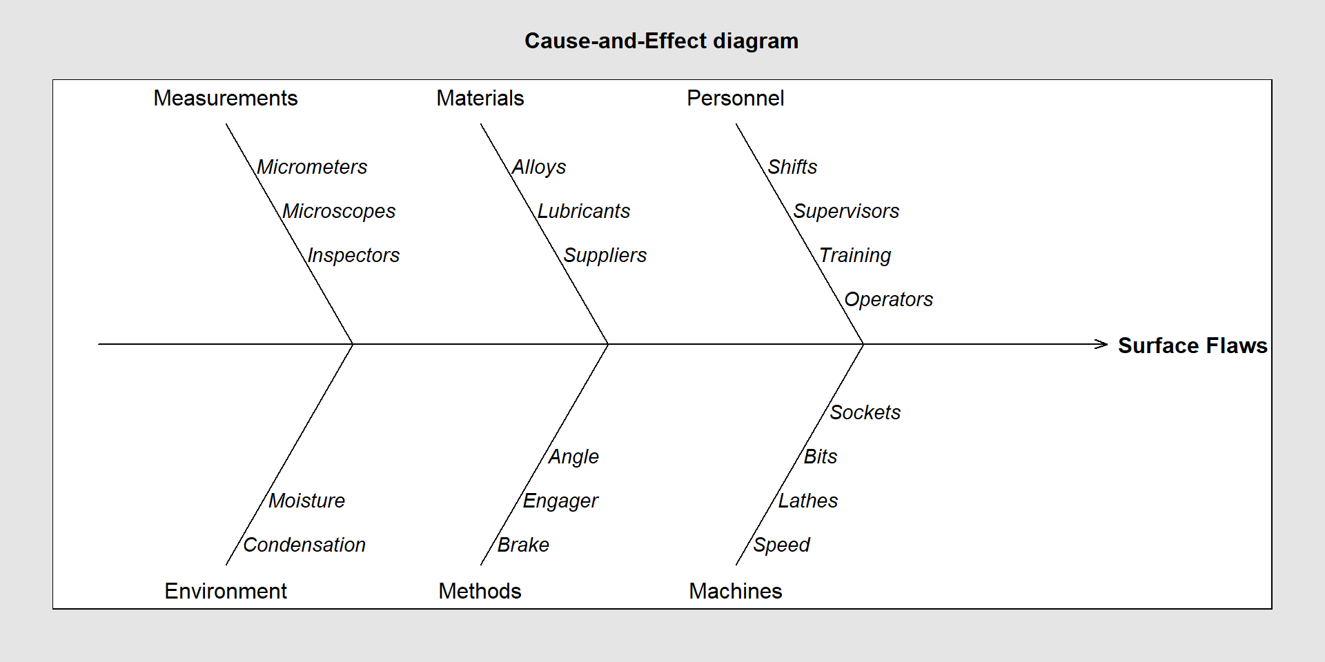
cause.and.effect(cause=list(Measurements=c("Micrometers", "Microscopes", "Inspectors"),
Materials=c("Alloys", "Lubricants", "Suppliers"),
Personnel=c("Shifts", "Supervisors", "Training", "Operators"),
Environment=c("Condensation", "Moisture"),
Methods=c("Brake", "Engager", "Angle"),
Machines=c("Speed", "Lathes", "Bits", "Sockets")),
effect="Surface Flaws")DSC 3091- Advanced Statistics Applications I
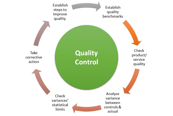
Statistical quality control
Department of Statistics and Computer Science
The process of using statistical tools and techniques to monitor and manage product quality across various industries.
Can be conducted as
A part of production process,
A part of last-minute quality control check
A part of eventual check by quality control department
![]()
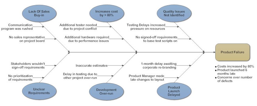
Cause and effect diagrams
is a visualization tool for categorizing the potential causes of a problem.
It can also be useful for showing relationships between contributing factors.
![]()
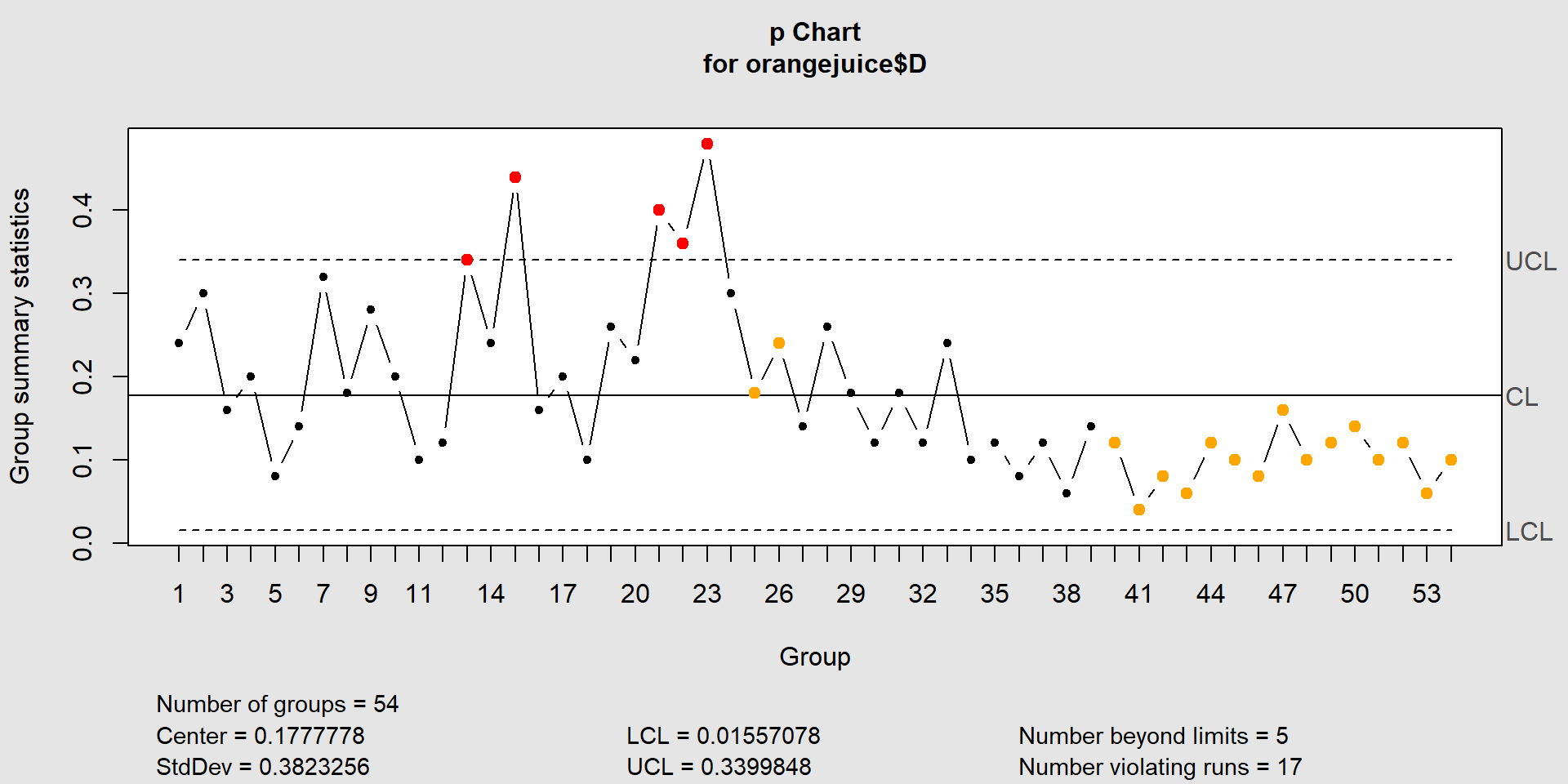
- The control limits are calculated based on the expected random variation in the process.
- The upper control limit (UCL) is 3 standard deviations above the center line.
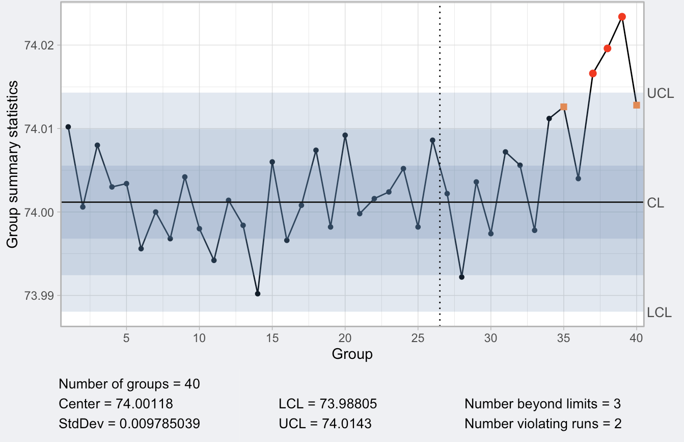
The lower control limit (LCL) is 3 standard deviations below the center line.
If a process is in control, all points on the control chart are between the upper and lower control limits.
Exercise 1
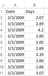
The quality.csv file contains data about time taken to deliver some products of Western shipping center in Colombo. The manager of the Western shipping center obtained this dataset by randomly selecting 10 samples for 20 days. Using the data, determine whether the delivery process of the company is stable over time.
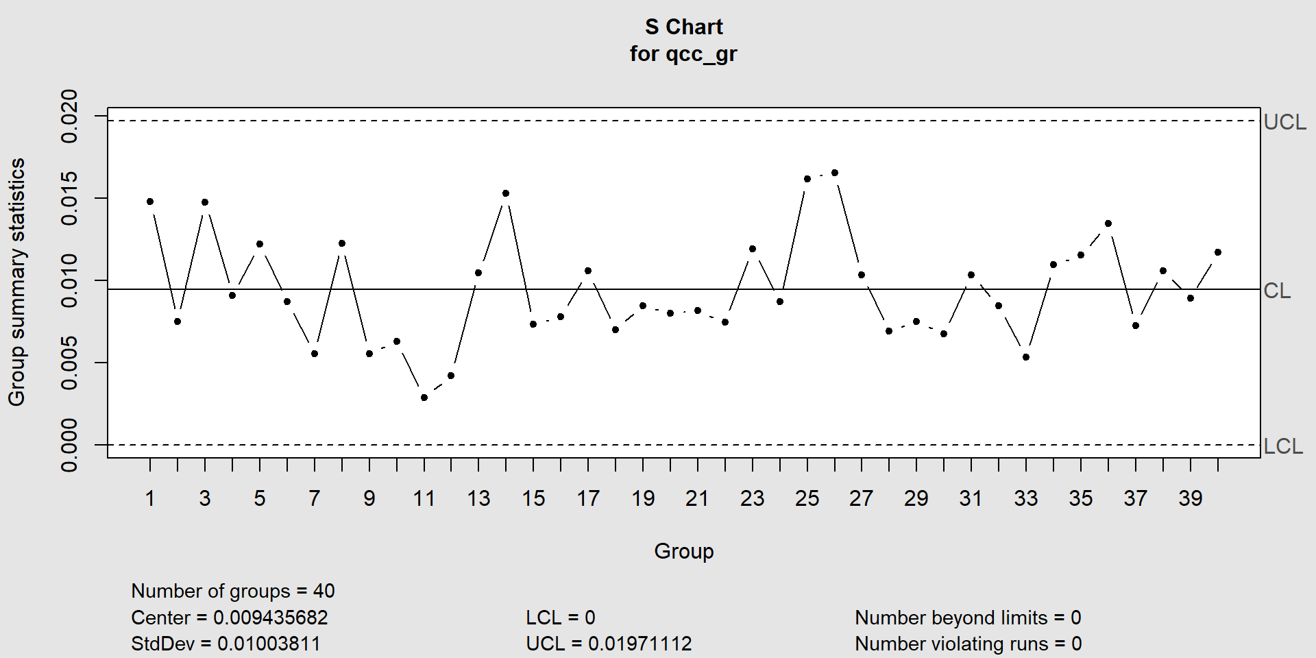
Create an S chart
- Use to assess the variability of the process.
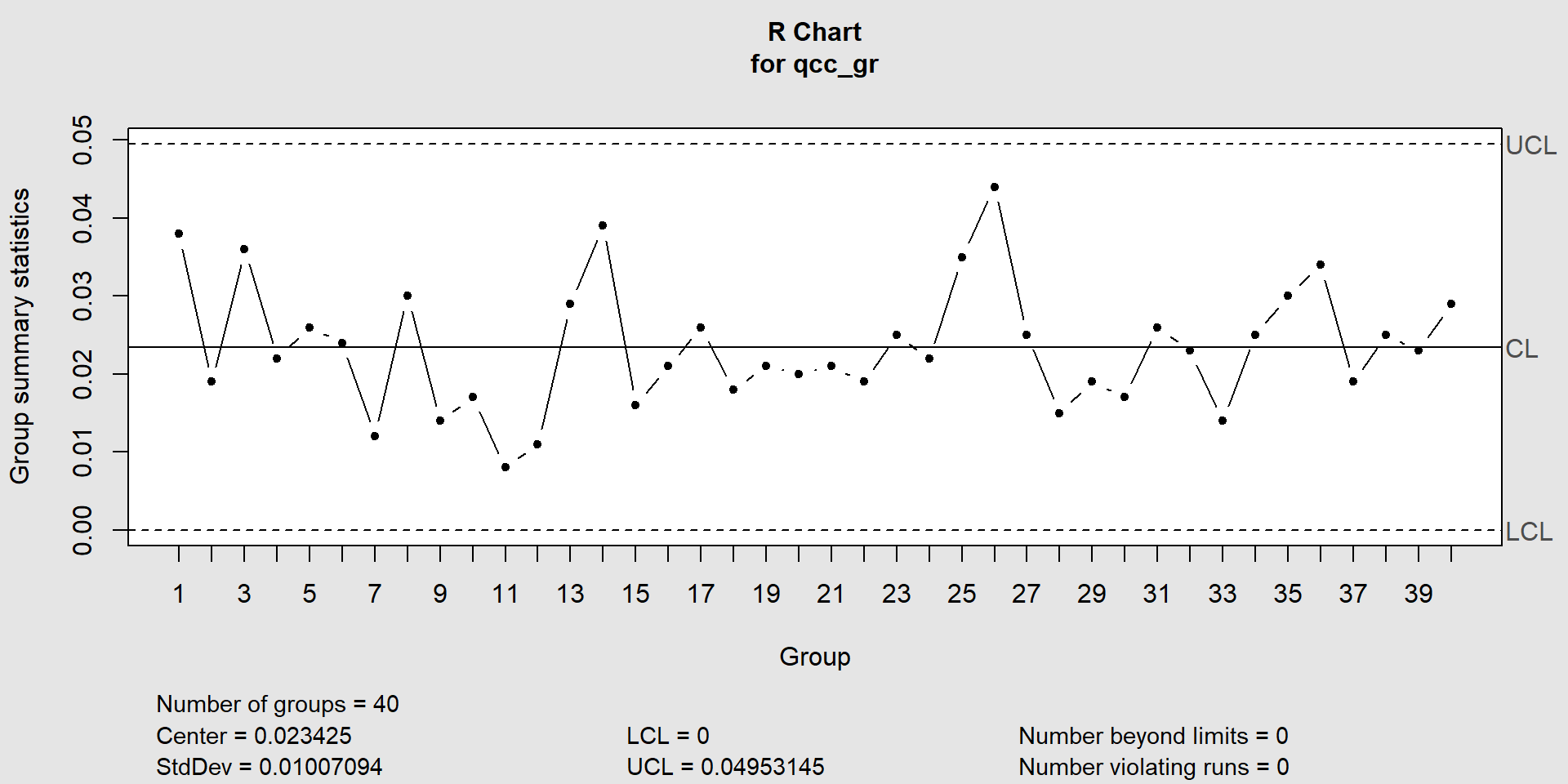
Create an R chart
- Use to assess the variability of the process with small samples.
Process capability analysis
- Measure whether consumer specified upper and lower specification limits (LSL/USL) are compatible with process control limits (LCL/UCL)
data(pistonrings)
attach(pistonrings)
diameter <- qcc.groups(diameter, sample)
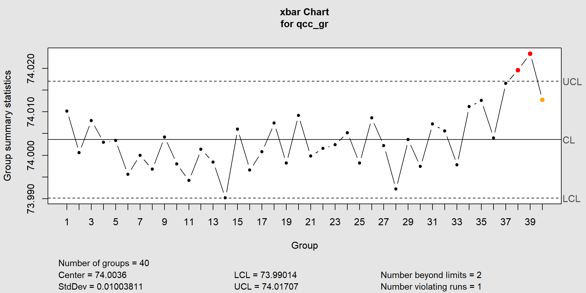
q <- qcc(diameter[1:25,], type="xbar", nsigmas=3, plot=FALSE)
process.capability(q, spec.limits=c(73.95,74.05))
Process Capability Analysis

Call:
process.capability(object = q, spec.limits = c(73.95, 74.05))

Number of obs = 125          Target = 74
       Center = 74              LSL = 73.95
       StdDev = 0.009785        USL = 74.05

Capability indices:

      Value   2.5%  97.5%
Cp    1.703  1.491  1.915
Cp_l  1.743  1.555  1.932
Cp_u  1.663  1.483  1.844
Cp_k  1.663  1.448  1.878
Cpm   1.691  1.480  1.902

Exp<LSL 0%   Obs<LSL 0%
Exp>USL 0%   Obs>USL 0%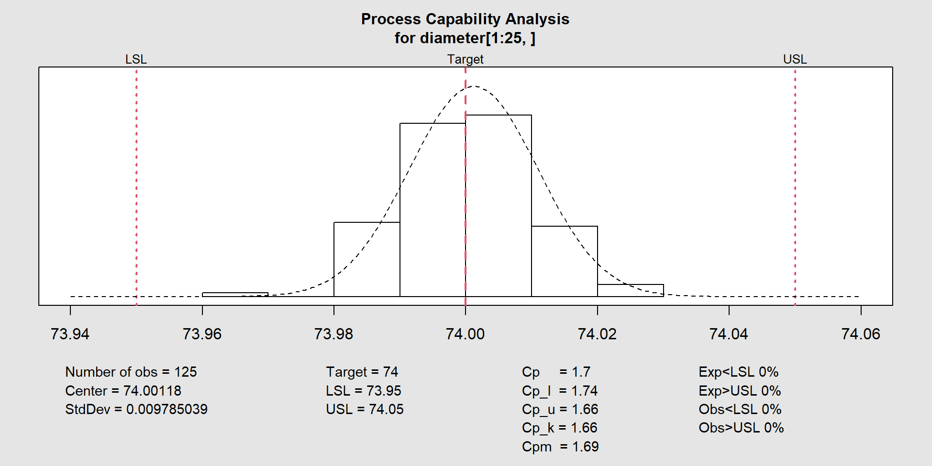
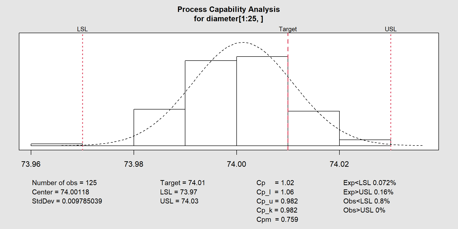
Process Capability Analysis

Call:
process.capability(object = q, spec.limits = c(73.97, 74.03),     target = 74.01)

Number of obs = 125          Target = 74.01
       Center = 74              LSL = 73.97
       StdDev = 0.009785        USL = 74.03

Capability indices:

       Value    2.5%   97.5%
Cp    1.0220  0.8948  1.1489
Cp_l  1.0620  0.9407  1.1833
Cp_u  0.9819  0.8682  1.0956
Cp_k  0.9819  0.8464  1.1174
Cpm   0.7589  0.6458  0.8719

Exp<LSL 0.072%   Obs<LSL 0.8%
Exp>USL 0.16%    Obs>USL 0%