class: center, inverse2 ### DSC3091 - Advanced Statistical application I # Introduction to Report writing with R .center[] --- class: middle ## EXPECTATION OF THE CLASS - Not to become an expert in all statistical software packages but to become an expert data scientist - Present an overview of what solutions are available with the emphasis on free open source software - Develop the skill set necessary to perform key aspects of data science efficiently. - The course covers the application of basic and advanced concepts in the R programming environment to allow a scalable implementation. <br/> <br/> ## Course Evaluation - Continuous Assesments (Mid Exam/Assignments): 40% - End Semester Examination: 60% --- class: middle # Code movies or Flipbooks - Flipbooks shows how to get from ‘A’ to ‘B’ in data manipulation, analysis, or visualization code pipelines. - Using flipbookr package you can present your code step-by-step and side-by-side with its output. - Together with the R package 'xaringan', flipbookr does four things: 1. Parses an .Rmd code pipeline from the chunk you indicate 2. Identifies break points in that code chunk pipeline 3. Spawns a bunch of code chunks with these partial builds of code, separated by slide breaks, and 4. Displays partial code in HTML slides. <br/> <br/> # Example --- count: false .panel1-slide1-auto[ ```r *set.seed(12345) ``` ] .panel2-slide1-auto[ ] --- count: false .panel1-slide1-auto[ ```r set.seed(12345) *library(tidyverse) ``` ] .panel2-slide1-auto[ ] --- count: false .panel1-slide1-auto[ ```r set.seed(12345) library(tidyverse) *mtcars ``` ] .panel2-slide1-auto[ ``` mpg cyl disp hp drat wt qsec vs am gear carb Mazda RX4 21.0 6 160.0 110 3.90 2.620 16.46 0 1 4 4 Mazda RX4 Wag 21.0 6 160.0 110 3.90 2.875 17.02 0 1 4 4 Datsun 710 22.8 4 108.0 93 3.85 2.320 18.61 1 1 4 1 Hornet 4 Drive 21.4 6 258.0 110 3.08 3.215 19.44 1 0 3 1 Hornet Sportabout 18.7 8 360.0 175 3.15 3.440 17.02 0 0 3 2 Valiant 18.1 6 225.0 105 2.76 3.460 20.22 1 0 3 1 Duster 360 14.3 8 360.0 245 3.21 3.570 15.84 0 0 3 4 Merc 240D 24.4 4 146.7 62 3.69 3.190 20.00 1 0 4 2 Merc 230 22.8 4 140.8 95 3.92 3.150 22.90 1 0 4 2 Merc 280 19.2 6 167.6 123 3.92 3.440 18.30 1 0 4 4 Merc 280C 17.8 6 167.6 123 3.92 3.440 18.90 1 0 4 4 Merc 450SE 16.4 8 275.8 180 3.07 4.070 17.40 0 0 3 3 Merc 450SL 17.3 8 275.8 180 3.07 3.730 17.60 0 0 3 3 Merc 450SLC 15.2 8 275.8 180 3.07 3.780 18.00 0 0 3 3 Cadillac Fleetwood 10.4 8 472.0 205 2.93 5.250 17.98 0 0 3 4 Lincoln Continental 10.4 8 460.0 215 3.00 5.424 17.82 0 0 3 4 Chrysler Imperial 14.7 8 440.0 230 3.23 5.345 17.42 0 0 3 4 Fiat 128 32.4 4 78.7 66 4.08 2.200 19.47 1 1 4 1 Honda Civic 30.4 4 75.7 52 4.93 1.615 18.52 1 1 4 2 Toyota Corolla 33.9 4 71.1 65 4.22 1.835 19.90 1 1 4 1 Toyota Corona 21.5 4 120.1 97 3.70 2.465 20.01 1 0 3 1 Dodge Challenger 15.5 8 318.0 150 2.76 3.520 16.87 0 0 3 2 AMC Javelin 15.2 8 304.0 150 3.15 3.435 17.30 0 0 3 2 Camaro Z28 13.3 8 350.0 245 3.73 3.840 15.41 0 0 3 4 Pontiac Firebird 19.2 8 400.0 175 3.08 3.845 17.05 0 0 3 2 Fiat X1-9 27.3 4 79.0 66 4.08 1.935 18.90 1 1 4 1 Porsche 914-2 26.0 4 120.3 91 4.43 2.140 16.70 0 1 5 2 Lotus Europa 30.4 4 95.1 113 3.77 1.513 16.90 1 1 5 2 Ford Pantera L 15.8 8 351.0 264 4.22 3.170 14.50 0 1 5 4 Ferrari Dino 19.7 6 145.0 175 3.62 2.770 15.50 0 1 5 6 Maserati Bora 15.0 8 301.0 335 3.54 3.570 14.60 0 1 5 8 Volvo 142E 21.4 4 121.0 109 4.11 2.780 18.60 1 1 4 2 ``` ] --- count: false .panel1-slide1-auto[ ```r set.seed(12345) library(tidyverse) mtcars %>% * rownames_to_column(var = "model") ``` ] .panel2-slide1-auto[ ``` model mpg cyl disp hp drat wt qsec vs am gear carb 1 Mazda RX4 21.0 6 160.0 110 3.90 2.620 16.46 0 1 4 4 2 Mazda RX4 Wag 21.0 6 160.0 110 3.90 2.875 17.02 0 1 4 4 3 Datsun 710 22.8 4 108.0 93 3.85 2.320 18.61 1 1 4 1 4 Hornet 4 Drive 21.4 6 258.0 110 3.08 3.215 19.44 1 0 3 1 5 Hornet Sportabout 18.7 8 360.0 175 3.15 3.440 17.02 0 0 3 2 6 Valiant 18.1 6 225.0 105 2.76 3.460 20.22 1 0 3 1 7 Duster 360 14.3 8 360.0 245 3.21 3.570 15.84 0 0 3 4 8 Merc 240D 24.4 4 146.7 62 3.69 3.190 20.00 1 0 4 2 9 Merc 230 22.8 4 140.8 95 3.92 3.150 22.90 1 0 4 2 10 Merc 280 19.2 6 167.6 123 3.92 3.440 18.30 1 0 4 4 11 Merc 280C 17.8 6 167.6 123 3.92 3.440 18.90 1 0 4 4 12 Merc 450SE 16.4 8 275.8 180 3.07 4.070 17.40 0 0 3 3 13 Merc 450SL 17.3 8 275.8 180 3.07 3.730 17.60 0 0 3 3 14 Merc 450SLC 15.2 8 275.8 180 3.07 3.780 18.00 0 0 3 3 15 Cadillac Fleetwood 10.4 8 472.0 205 2.93 5.250 17.98 0 0 3 4 16 Lincoln Continental 10.4 8 460.0 215 3.00 5.424 17.82 0 0 3 4 17 Chrysler Imperial 14.7 8 440.0 230 3.23 5.345 17.42 0 0 3 4 18 Fiat 128 32.4 4 78.7 66 4.08 2.200 19.47 1 1 4 1 19 Honda Civic 30.4 4 75.7 52 4.93 1.615 18.52 1 1 4 2 20 Toyota Corolla 33.9 4 71.1 65 4.22 1.835 19.90 1 1 4 1 21 Toyota Corona 21.5 4 120.1 97 3.70 2.465 20.01 1 0 3 1 22 Dodge Challenger 15.5 8 318.0 150 2.76 3.520 16.87 0 0 3 2 23 AMC Javelin 15.2 8 304.0 150 3.15 3.435 17.30 0 0 3 2 24 Camaro Z28 13.3 8 350.0 245 3.73 3.840 15.41 0 0 3 4 25 Pontiac Firebird 19.2 8 400.0 175 3.08 3.845 17.05 0 0 3 2 26 Fiat X1-9 27.3 4 79.0 66 4.08 1.935 18.90 1 1 4 1 27 Porsche 914-2 26.0 4 120.3 91 4.43 2.140 16.70 0 1 5 2 28 Lotus Europa 30.4 4 95.1 113 3.77 1.513 16.90 1 1 5 2 29 Ford Pantera L 15.8 8 351.0 264 4.22 3.170 14.50 0 1 5 4 30 Ferrari Dino 19.7 6 145.0 175 3.62 2.770 15.50 0 1 5 6 31 Maserati Bora 15.0 8 301.0 335 3.54 3.570 14.60 0 1 5 8 32 Volvo 142E 21.4 4 121.0 109 4.11 2.780 18.60 1 1 4 2 ``` ] --- count: false .panel1-slide1-auto[ ```r set.seed(12345) library(tidyverse) mtcars %>% rownames_to_column(var = "model") %>% * ggplot() ``` ] .panel2-slide1-auto[ <!-- --> ] --- count: false .panel1-slide1-auto[ ```r set.seed(12345) library(tidyverse) mtcars %>% rownames_to_column(var = "model") %>% ggplot() + * aes(x = wt * 1000) ``` ] .panel2-slide1-auto[ 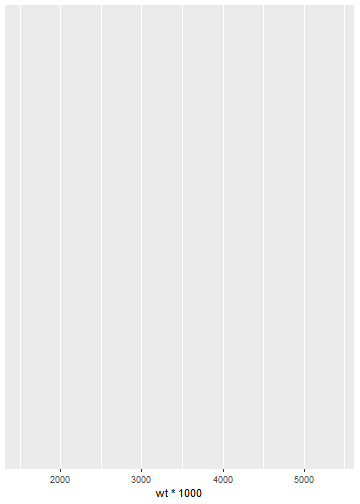<!-- --> ] --- count: false .panel1-slide1-auto[ ```r set.seed(12345) library(tidyverse) mtcars %>% rownames_to_column(var = "model") %>% ggplot() + aes(x = wt * 1000) + * aes(y = factor(cyl)) ``` ] .panel2-slide1-auto[ 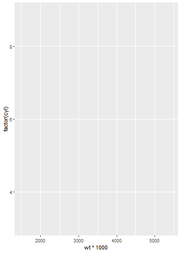<!-- --> ] --- count: false .panel1-slide1-auto[ ```r set.seed(12345) library(tidyverse) mtcars %>% rownames_to_column(var = "model") %>% ggplot() + aes(x = wt * 1000) + aes(y = factor(cyl)) + * ggthemes::theme_solarized() ``` ] .panel2-slide1-auto[ 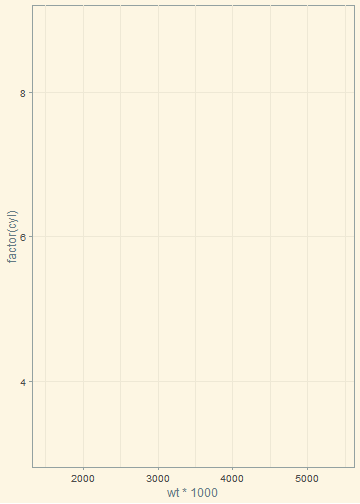<!-- --> ] --- count: false .panel1-slide1-auto[ ```r set.seed(12345) library(tidyverse) mtcars %>% rownames_to_column(var = "model") %>% ggplot() + aes(x = wt * 1000) + aes(y = factor(cyl)) + ggthemes::theme_solarized() + * geom_boxplot(fill = "snow2") ``` ] .panel2-slide1-auto[ <!-- --> ] --- count: false .panel1-slide1-auto[ ```r set.seed(12345) library(tidyverse) mtcars %>% rownames_to_column(var = "model") %>% ggplot() + aes(x = wt * 1000) + aes(y = factor(cyl)) + ggthemes::theme_solarized() + geom_boxplot(fill = "snow2") + * geom_jitter(height = .2, alpha = .8, * color = "plum3", size = 3) ``` ] .panel2-slide1-auto[ <!-- --> ] --- count: false .panel1-slide1-auto[ ```r set.seed(12345) library(tidyverse) mtcars %>% rownames_to_column(var = "model") %>% ggplot() + aes(x = wt * 1000) + aes(y = factor(cyl)) + ggthemes::theme_solarized() + geom_boxplot(fill = "snow2") + geom_jitter(height = .2, alpha = .8, color = "plum3", size = 3) + * labs(y = "Number of Cylinders") ``` ] .panel2-slide1-auto[ 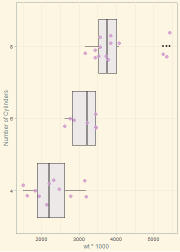<!-- --> ] --- count: false .panel1-slide1-auto[ ```r set.seed(12345) library(tidyverse) mtcars %>% rownames_to_column(var = "model") %>% ggplot() + aes(x = wt * 1000) + aes(y = factor(cyl)) + ggthemes::theme_solarized() + geom_boxplot(fill = "snow2") + geom_jitter(height = .2, alpha = .8, color = "plum3", size = 3) + labs(y = "Number of Cylinders") + * labs(x = "Weight in pounds") ``` ] .panel2-slide1-auto[ 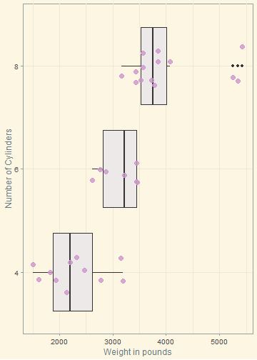<!-- --> ] --- count: false .panel1-slide1-auto[ ```r set.seed(12345) library(tidyverse) mtcars %>% rownames_to_column(var = "model") %>% ggplot() + aes(x = wt * 1000) + aes(y = factor(cyl)) + ggthemes::theme_solarized() + geom_boxplot(fill = "snow2") + geom_jitter(height = .2, alpha = .8, color = "plum3", size = 3) + labs(y = "Number of Cylinders") + labs(x = "Weight in pounds") + * labs(title = "How do number of cylinders and model weight relate?") ``` ] .panel2-slide1-auto[ 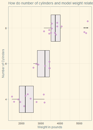<!-- --> ] --- count: false .panel1-slide1-auto[ ```r set.seed(12345) library(tidyverse) mtcars %>% rownames_to_column(var = "model") %>% ggplot() + aes(x = wt * 1000) + aes(y = factor(cyl)) + ggthemes::theme_solarized() + geom_boxplot(fill = "snow2") + geom_jitter(height = .2, alpha = .8, color = "plum3", size = 3) + labs(y = "Number of Cylinders") + labs(x = "Weight in pounds") + labs(title = "How do number of cylinders and model weight relate?") + * labs(subtitle = "Motor Trend US magazine's comparison of thirty-two 1973-74 models") ``` ] .panel2-slide1-auto[ 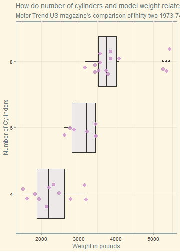<!-- --> ] --- count: false .panel1-slide1-auto[ ```r set.seed(12345) library(tidyverse) mtcars %>% rownames_to_column(var = "model") %>% ggplot() + aes(x = wt * 1000) + aes(y = factor(cyl)) + ggthemes::theme_solarized() + geom_boxplot(fill = "snow2") + geom_jitter(height = .2, alpha = .8, color = "plum3", size = 3) + labs(y = "Number of Cylinders") + labs(x = "Weight in pounds") + labs(title = "How do number of cylinders and model weight relate?") + labs(subtitle = "Motor Trend US magazine's comparison of thirty-two 1973-74 models") + * theme(plot.title.position = "plot") ``` ] .panel2-slide1-auto[ 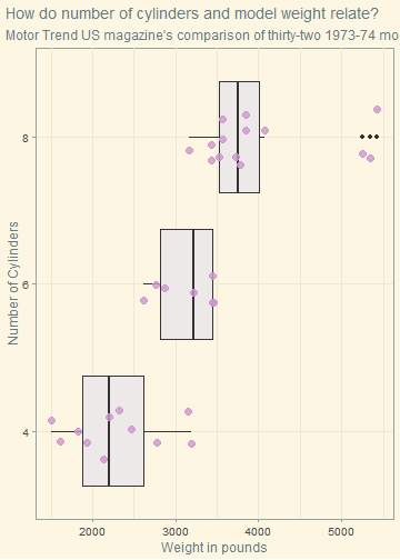<!-- --> ] <style> .panel1-slide1-auto { color: black; width: 38.6060606060606%; hight: 32%; float: left; padding-left: 1%; font-size: 80% } .panel2-slide1-auto { color: black; width: 59.3939393939394%; hight: 32%; float: left; padding-left: 1%; font-size: 80% } .panel3-slide1-auto { color: black; width: NA%; hight: 33%; float: left; padding-left: 1%; font-size: 80% } </style> --- # Create your own flipbook - After installing flipbookr with `install.packages("flipbookr")` or `devtools::install_github("EvaMaeRey/flipbookr"),` we can use the following menu commands to open a minimal flipbook. File -> New File -> R Markdown -> From Template -> A Minimal Flipbook - Further, you need `rmarkdown` and `Xaringan` packages, which you can download directly from CRAN. - The YAML meta data of this file given below presents an html {xaringan} slide show output. ``` title: "A minimal flipbook" subtitle: "With flipbookr and xaringan" author: "You!" output: xaringan::moon_reader: lib_dir: libs css: [default, hygge, ninjutsu] nature: ratio: 16:9 highlightStyle: github highlightLines: true countIncrementalSlides: false ``` --- class: middle # YAML meta data - `knit` the .Rmd file by giving a name. - Then, in the current folder, two new folders `libs` and `test_files` will be created. - The header attributes and CSS files are saved in the `libs` folder, and note that `libs` is the folder name that we have specified in the lib_dir in YAML. - The figures relevant to this `test.Rmd` are saved in the test_files folder. - The three CSS files mentioned in YAML are, 1. `default` - default CSS for formatting xaringan \ 2. `hygge` - CSS for further formatting xaringan \ 3. `ninjutsu` - CSS for the theme for slides. - The ratio in YAML gives the width and height of the slides. - The option `highlightLines:true` of nature will highlight code lines, and `highlightStyle:github` use the specific style. - Setting the option `countIncrementalSlides:false` will not be displayed a number when each slide is incremented with each new slide. --- class: middle # The setup chunk in .Rmd file ``` # This is the recommended set up for flipbooks # you might think about setting cache to TRUE as you gain practice --- building flipbooks from scratch can be time consuming knitr::opts_chunk$set(fig.width = 6, message = FALSE, warning = FALSE, comment = "", cache = F) library(flipbookr) library(tidyverse) ``` <br/> - Here, we specify the relevant options to ignore showing messages, warnings or comments in slides when running R codes. - We can also set up the width of the figures. - We can specify to load {flipbookr}, and other packages that you need for your presentation in this setup chunk. --- # Create a 'source' code chunk with a code pipeline - A source code chunk, named 'my_cars' .left[] - In your .Rmd use the {flipbookr} function `chunk_reveal()` inline as follows. Refer to the source code chunk that you have prepared by name. .left[] --- count: false ### First flipbook .panel1-my_cars-auto[ ```r *cars ``` ] .panel2-my_cars-auto[ ``` speed dist 1 4 2 2 4 10 3 7 4 4 7 22 5 8 16 6 9 10 7 10 18 8 10 26 9 10 34 10 11 17 11 11 28 12 12 14 13 12 20 14 12 24 15 12 28 16 13 26 17 13 34 18 13 34 19 13 46 20 14 26 21 14 36 22 14 60 23 14 80 24 15 20 25 15 26 26 15 54 27 16 32 28 16 40 29 17 32 30 17 40 31 17 50 32 18 42 33 18 56 34 18 76 35 18 84 36 19 36 37 19 46 38 19 68 39 20 32 40 20 48 41 20 52 42 20 56 43 20 64 44 22 66 45 23 54 46 24 70 47 24 92 48 24 93 49 24 120 50 25 85 ``` ] --- count: false ### First flipbook .panel1-my_cars-auto[ ```r cars %>% * filter(speed > 4) ``` ] .panel2-my_cars-auto[ ``` speed dist 1 7 4 2 7 22 3 8 16 4 9 10 5 10 18 6 10 26 7 10 34 8 11 17 9 11 28 10 12 14 11 12 20 12 12 24 13 12 28 14 13 26 15 13 34 16 13 34 17 13 46 18 14 26 19 14 36 20 14 60 21 14 80 22 15 20 23 15 26 24 15 54 25 16 32 26 16 40 27 17 32 28 17 40 29 17 50 30 18 42 31 18 56 32 18 76 33 18 84 34 19 36 35 19 46 36 19 68 37 20 32 38 20 48 39 20 52 40 20 56 41 20 64 42 22 66 43 23 54 44 24 70 45 24 92 46 24 93 47 24 120 48 25 85 ``` ] --- count: false ### First flipbook .panel1-my_cars-auto[ ```r cars %>% filter(speed > 4) %>% * ggplot() ``` ] .panel2-my_cars-auto[ <!-- --> ] --- count: false ### First flipbook .panel1-my_cars-auto[ ```r cars %>% filter(speed > 4) %>% ggplot() + * aes(x = speed) ``` ] .panel2-my_cars-auto[ <!-- --> ] --- count: false ### First flipbook .panel1-my_cars-auto[ ```r cars %>% filter(speed > 4) %>% ggplot() + aes(x = speed) + * aes(y = dist) ``` ] .panel2-my_cars-auto[ <!-- --> ] --- count: false ### First flipbook .panel1-my_cars-auto[ ```r cars %>% filter(speed > 4) %>% ggplot() + aes(x = speed) + aes(y = dist) + * geom_point( * alpha = .8, * color = "blue" * ) ``` ] .panel2-my_cars-auto[ 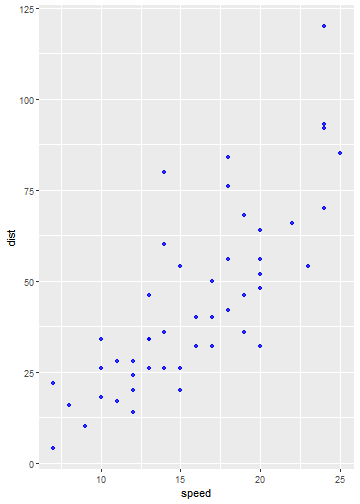<!-- --> ] --- count: false ### First flipbook .panel1-my_cars-auto[ ```r cars %>% filter(speed > 4) %>% ggplot() + aes(x = speed) + aes(y = dist) + geom_point( alpha = .8, color = "blue" ) + * aes(size = speed) ``` ] .panel2-my_cars-auto[ 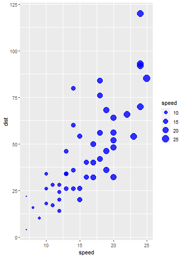<!-- --> ] <style> .panel1-my_cars-auto { color: black; width: 38.6060606060606%; hight: 32%; float: left; padding-left: 1%; font-size: 80% } .panel2-my_cars-auto { color: black; width: 59.3939393939394%; hight: 32%; float: left; padding-left: 1%; font-size: 80% } .panel3-my_cars-auto { color: black; width: NA%; hight: 33%; float: left; padding-left: 1%; font-size: 80% } </style> - Also, indicate you want a slide break before the inline code as shown above. The slide break is indicated with three dashes, '---' at the beginning of a line with no trailing spaces. --- class: center middle inverse2 # Let's Try Out! --- # How to define the break points? - There are several ways that input code can be revealed: * auto * user * non_seq * rotate * 5 (set to an integer) ``` cars %>% filter(speed > 4) %>% ggplot() + aes(x = speed) + #BREAK aes(y = dist) + #BREAK geom_point( alpha = .8, color = "blue" ) + aes(size = speed) #BREAK ``` - In the above code, notice the `#BREAK` comments, these will be used for a couple of the different break_type modes. --- class: middle - `break_type = "auto"` The default break_type is "auto", in which appropriate breakpoints are determined automatically --- by finding where parentheses are balanced. - `break_type = "user"`, with #BREAK If the break_type is set to "user", the breakpoints are those indicated by the user with the special comment #BREAK - `break_type = "non_seq"`, with #BREAK2, #BREAK3 If the break_type is set to "non_seq", the breakpoints are those indicated by the user with the special numeric comment #BREAK2, #BREAK3 etc to indicate at which point in time the code should appear. - `break_type = "rotate"` And break_type = "rotate" is used to to cycle through distinct lines of code. The special comment to indicate which lines should be cycled through is #ROTATE. More details: https://evamaerey.github.io/flipbooks/flipbook_recipes#48 --- count: false ### Second flipbook .panel1-my_cars2-user[ ```r *cars %>% * filter(speed > 4) %>% * ggplot() + * aes(x = speed) ``` ] .panel2-my_cars2-user[ <!-- --> ] --- count: false ### Second flipbook .panel1-my_cars2-user[ ```r cars %>% filter(speed > 4) %>% ggplot() + aes(x = speed) + * aes(y = dist) ``` ] .panel2-my_cars2-user[ <!-- --> ] --- count: false ### Second flipbook .panel1-my_cars2-user[ ```r cars %>% filter(speed > 4) %>% ggplot() + aes(x = speed) + aes(y = dist) + * geom_point( * alpha = .8, * color = "blue" * ) + * aes(size = speed) ``` ] .panel2-my_cars2-user[ <!-- --> ] <style> .panel1-my_cars2-user { color: black; width: 38.6060606060606%; hight: 32%; float: left; padding-left: 1%; font-size: 80% } .panel2-my_cars2-user { color: black; width: 59.3939393939394%; hight: 32%; float: left; padding-left: 1%; font-size: 80% } .panel3-my_cars2-user { color: black; width: NA%; hight: 33%; float: left; padding-left: 1%; font-size: 80% } </style> --- class: center middle inverse2 # Quarto Documents --- # Quarto Documents - Quarto is a multi-language, next-generation version of R Markdown from RStudio. - Includes dozens of new features and capabilities while at the same being able to render most existing Rmd files without modification. - Quarto documents are saved with the .qmd extension, and can be rendered as HTML file. - You could also choose to render it into other formats like PDF, MS Word, etc. .center[] --- # Let's Get Started! - Download and install the latest release of RStudio (v2022.02+) - Download the quarto library from the link below https://quarto.org/docs/get-started/ - Once you install it, choose your tool and get started .center[] - Be sure that you have installed the `tidyverse` and `palmerpenguins` packages ``` install.packages("tidyverse") install.packages("palmerpenguins") ``` - Open the `hello.qmd` in your working directory in RStudio, and click on Render --- # Rendering - Use the `Render` button in the RStudio IDE to render the file and preview the output with a single click or keyboard shortcut (Ctrl+Shift+K). <img src="images/render1.png" width="800px" /> - If you prefer to automatically render whenever you save, you can check the Render on Save option on the editor toolbar. <img src="images/render2.png" width="800px" /> - The preview will update whenever you re-render the document. Side-by-side preview works for both HTML and PDF outputs. <img src="images/render3.png" width="800px" /> --- class: middle # Authoring - RStudio editor contains two modes of the same quarto document: visual and source - Visual editor offers an `WYSIWYM` authoring experience for markdown. - The source code of the same document is written for you and you can view/edit it at any point by switching to source mode for editing. - You can toggle back and forth these two modes by clicking on Source and Visual in the editor toolbar. --- # Contents of a Quarto document - A Quarto document contains three types of content: 1. a YAML header, 2. code chunks, and 3. markdown text. ## YAML header ``` --- title: "Hello, Quarto" format: html editor: visual --- ``` - When rendered, the title , "Hello, Quarto", will appear at the top of the rendered document with a larger font size - The other two YAML fields in denote that the output should be in html format and the document should open in the visual editor - The basic syntax of YAML uses key-value pairs in the format `key: value`. - Other YAML fields commonly found in headers of documents include metadata like `author, subtitle, date` as well as customization options like `theme, fontcolor, fig-width`, etc. --- ## Code chunks - R code chunks identified with `{r}` with (optional) chunk options. - Chunk options can be defined by `#|` at the beginning of the line. <!-- --> ## Markdown text - Quarto uses markdown syntax for text. - If using the visual editor, you can use the menus and shortcuts to add a header, bold text, insert a table, etc. --- # Computations - For some documents, you may want to hide all of the code and just show the output. To do so, specify `echo: false` within the `execute` option in the YAML. --- title: "Quarto Computations" execute: echo: false --- - To selectively enable code echo for some cells, add the `echo: true` cell option. ``` #| label: scatterplot #| echo: true ggplot(mpg, aes(x = hwy, y = cty, color = cyl)) + geom_point(alpha = 0.5, size = 2) + scale_color_viridis_c() + theme_minimal() ``` --- # Code Folding - Rather than hiding code entirely, you might want to fold it and allow readers to view it at their discretion. - You can do this via the code-fold option. - Remove the `echo` option we previously added and add the `code-fold` HTML format option. --- title: "Quarto Computations" format: html: code-fold: true --- - You can also provide global control over code folding. Try adding `code-tools: true` to the HTML --- # Code Linking - The code-link option enables hyper-linking of functions within code blocks to their online documentation. - Try adding `code-link: true` to the HTML format options. --- title: "Quarto Computations" format: html: code-link: true --- - Note that code linking is currently implemented only for the knitr engine via the `downlit` package. --- # Caching - If your document includes code chunks that take too long to compute, you might want to cache the results of those chunks. - Use the cache option at the document level --- execute: cache: true --- - Use the cache option for a particular chunk --- #| cache: true --- --- # Inline Code - To include executable expressions within markdown, enclose the expression in ``` `r ` ``` - Eg: There are 'r nrow(mpg)` observations in our data. --- There are 234 observations in our data. --- - If the expression you want to inline is more complex, it is recommend including it in a code chunk (with `echo: false`) #| echo: false mean_cty <- round(mean(mpg$cty), 2) mean_hwy <- round(mean(mpg$hwy), 2) - Then, add the following markdown text to your Quarto document. The average city mileage of the cars in our data is 16.86 and the average highway mileage is 23.44. --- # Data Frames - You can control how data frames are printed by default using the df-print document option. Available options include: <img src="images/Data_frames.png" width="800px" /> --- title: "Document" format: html: df-print: paged --- --- # Figures - We can improve the appearance and accessibility of our plot. - We can change its aspect ratio by setting `fig-width` and `fig-height`, provide a `fig-cap`, modify its `label` for cross referencing, and add alternative text with `fig-alt`. --- #| label: fig-scatterplot #| fig-cap: "City and highway mileage for 38 popular models of cars." #| fig-alt: "Scatterplot of city vs. highway mileage for cars, where points are colored by the number of cylinders. The plot displays a positive, linear, and strong relationship between city and highway mileage, and mileage increases as the number cylinders decreases." #| fig-width: 6 #| fig-height: 3.5 --- @fig-scatterplot shows a positive, strong, and linear relationship between the city and highway mileage of these cars. --- # Multiple Figures - We can use `layout-ncol` option to display the plots side-by-side. --- #| label: fig-mpg #| fig-cap: "City and highway mileage for 38 popular models of cars." #| fig-subcap: #| - "Color by number of cylinders" #| - "Color by engine displacement, in liters" #| layout-ncol: 2 #| column: page ggplot(mpg, aes(x = hwy, y = cty, color = cyl)) + geom_point(alpha = 0.5, size = 2) + scale_color_viridis_c() + theme_minimal() ggplot(mpg, aes(x = hwy, y = cty, color = displ)) + geom_point(alpha = 0.5, size = 2) + scale_color_viridis_c(option = "E") + theme_minimal() --- In `@fig-mpg-1` the points are colored by the number of cylinders while in `@fig-mpg-2` the points are colored by engine displacement. --- class: middle # More options to look at - Output Formats: Html, pdf and word - Multiple Formats: You can obtain multiple formats of the same document - Table of contents and section numbering - Equations - Citations - Cross References - Article Layout and Publishing Please refer the following tutorial to learn more: https://quarto.org/docs/get-started/authoring/ --- class: center middle inverse2 # Introduction to SWIRL --- class: middle # Swirl - an R package for teaching and learning statistics and R simultaneously and interactively. - Composed of: * text output, * multiple choice and text-based questions, and * questions that require the user to enter actual R code at the prompt. - Responses are evaluated for correctness based on instructor-specified answer tests, and appropriate feedback is given immediately to the user. - Install swirl package --- install.packages("swirl") --- --- # Start swirl - You will need to do this every time you start R or want to continue an old lesson or start a new lesson. --- # load the swirl package into your current R session library(swirl) | Hi! Type swirl() when you are ready to begin. swirl() --- - Choose a name --- What shall I call you? --- --- --- #Choose a course --- | To begin, you must install a course. I can install a course for you from the internet, | or I can send you to a web page (https://github.com/swirldev/swirl_courses) which will | provide course options and directions for installing courses yourself. (If you are not | connected to the internet, type 0 to exit.) 1: R Programming: The basics of programming in R 2: Regression Models: The basics of regression modeling in R 3: Statistical Inference: The basics of statistical inference in R 4: Exploratory Data Analysis: The basics of exploring data in R 5: Don't install anything for me. I'll do it myself. --- - Choose a lesson and do it. --- class: middle #Some useful commands for swirl - bye(): Exit swirl - play(): Leave swirl temporarily and gain access to the console again - nxt(): Return to swirl after playing - main(): Return to the main menu - info(): Display a list of these special commands --- class: middle # Some useful links 1. https://www.w3schools.io/file/markdown-blockquotes/ 2. https://evamaerey.github.io/flipbooks/flipbookr/skeleton#1 3. https://pushpa-wijekoon.netlify.app/ 4. https://quarto.org/docs/get-started/hello/rstudio.html 5. https://yihui.org/en/2022/04/quarto-r-markdown/ 6. https://www.apreshill.com/blog/2022-04-we-dont-talk-about-quarto/ 7. https://www.youtube.com/watch?v=6p4vOKS6Xls&feature=youtu.be 8. https://www.youtube.com/watch?v=shVSmYna3GM 9. https://www.r-bloggers.com/2017/01/why-swirl/ 10. https://swirlstats.com/ 11. http://www.simonqueenborough.info/R/basic/intro-to-swirl 12. https://www.coursera.org/lecture/r-programming/introduction-to-swirl-QLz9h 13. https://www.youtube.com/watch?v=vSKm8JyHBE0